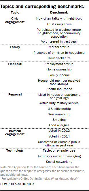
To understand the relative merits of alternative adjustment procedures, each was assessed on its effectiveness at reducing bias for 24 different benchmarks drawn from high-quality, “gold-standard” surveys. These benchmarks cover a range of topics including civic and political engagement (both difficult topics for surveys in general), technology use, personal finances, household composition and other personal characteristics. See Appendix D for a complete list. While these benchmarks all come from high-quality surveys, it is important to note that these measures are themselves estimates and are subject to error. As a result, the estimates of bias described here should be thought of as approximations.
For each simulated survey dataset with sample sizes ranging from 2,000 to 8,000, the seven statistical techniques were applied twice, once using only demographic variables, and once using both demographic and political variables. This produced a total of 14 different sets of weights for each dataset. Next, estimates were calculated for each substantive category17 of the 24 benchmark questions using each set of weights as well as unweighted.
The estimated bias for each category is the difference between the survey estimate and the benchmark value.18 To summarize the level of bias for all of the categories of a particular benchmark variable, we calculated the average of the absolute values of the estimated biases for each of the variable’s categories. To summarize the overall level of bias across multiple questions (e.g., all 24 benchmarks), the average of the question-level averages was used.
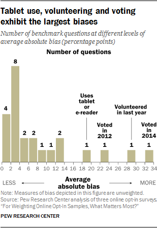
Prior to any weighting, the estimated average absolute bias for the 24 benchmark variables was 8.4 percentage points. Many of the estimated biases are relatively small. Half of the variables have average biases under 4 points, four of which are under 2 points (family income, home ownership, marital status and health insurance coverage). At the other end of the scale, four variables show extremely large biases. These are voting in the 2014 midterm election, (32 percentage points), having volunteered in the past 12 months (29 points), voting in the 2012 presidential election (23 points) and tablet ownership (20 points).
Choice of variables for weighting is more consequential than the statistical method
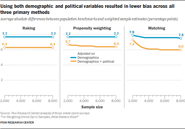
More than any other factor, the choice of adjustment variables has the largest impact on the accuracy of estimates. Adjusting on both the demographic and political variables resulted in lower average bias than adjusting on demographics alone. While the largest improvements were for measures of political engagement (such as voting), benchmarks related to civic engagement and technology use also saw sizable reductions in bias. The differences between survey topics are examined in detail in the section “Choice of adjustment variables has a much larger impact when related to the survey topic.”
This was true for all three primary statistical methods as well as the four combination methods, and it was true at every sample size. On average, adjusting on demographics alone reduced estimated bias by just under 1 percentage point, from 8.4 points before weighting to 7.6 after. This effect was relatively consistent regardless of the statistical method or sample size. By contrast, weighting on both demographics and the political variables reduces bias an additional 1.4 percentage points on average, although the degree of improvement was more sensitive to the statistical method and sample size. Under the best-case scenario, the more comprehensive set of adjustment variables reduced the average estimated bias to a low of 6 percentage points.
Matching on its own can improve upon raking, but only modestly and with large samples
The study examined how the performance of each adjustment method is affected by sample size. For raking, the reduction in bias was effectively the same at every sample size. The average estimated bias with n=8,000 interviews is identical to that with n=2,000 interviews (7.7 percentage points when adjusting on demographics and 6.3 for demographic + political variables).
Matching, on the other hand, becomes more effective with larger starting sample sizes because there are more match candidates for each case in the target sample. When adjusting on demographic variables, matching did show a small improvement as the sample size increased, going from an average estimated bias of 7.9 percentage points at a starting sample size of n=2,000 to 7.5 points at n=8,000. When political variables were included in the adjustment, the benefits of a larger starting sample are more substantial, going from a high of 7.3 points at n=2,000 to a low of 6 points at n=8,000. Even so, matching reached a point of diminishing returns around n=4,000 and levels off completely at n=5,500 and greater. This suggests that that there may not be much benefit from further increasing the size of the starting sample when the target size is 1,500.
Most notably, matching by itself performed quite poorly relative to raking at smaller sample sizes. When n=2,000, raking’s average estimated bias was a full point lower for raking. Matching did not overtake raking until the starting sample size reached 3,500. At best, matching improved upon raking by a relatively modest 0.3 points, and then only at sample sizes of 5,500 or larger. None of the opt-in panel vendors that regularly employ matching use this approach on its own; rather, they follow matching with additional stages of adjustment or statistical modeling.
Unlike matching, propensity weighting was never more effective than raking. When only demographics were used, the estimated bias was equal to raking at a constant at 7.7 percentage points. With both demographic and political variables employed, propensity-weighting bias ranged from 6.7 points when n=2,000 to 6.4 points at n=8,000. This improvement likely occurs because the random forest algorithm used to estimate the propensities can fit more complex and powerful models given more data and more variables.
Raking in addition to matching or propensity weighting can be better than raking alone
When multiple techniques were used together in sequence, the result was slightly more bias correction than any of the methods on their own. At smaller starting sample sizes (e.g., n=less than 4,000), matching performed quite poorly relative to raking. But if both matching and raking were performed, the result was slightly lower bias than with raking alone. For example, when a starting sample of n=2,000 was matched on both demographic and political variables, the average estimated bias was 7.3 points, but when the matching was followed by raking, the average bias dropped to 6.2 points, putting it just ahead of raking by 0.1 point on average.
When matching was followed by propensity weighting, there was some improvement in accuracy, but not as much. A third stage of raking applied after propensity weighting produced the same results as just matching plus raking, suggesting that any added benefit from an intermediate propensity weighting step is minimal.
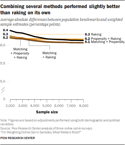
A similar pattern emerged when propensity weighting was followed by raking. On its own, propensity weighting always performed worse than raking, but when the two were used in combination with both demographic and political variables, the result was a small but consistent improvement of 0.1 points compared with raking alone. While there are few scenarios where matching or propensity weighting would be preferable to raking when used in isolation, they can add value when combined with raking. That being said, the benefits are very small, on the order of 0.1 percentage points, and may not be worth the extra effort.
Perhaps the most interesting finding was how little benefit came from having a large sample size. The most effective adjustment protocol reduced the average bias to 6 percentage points with a sample size of at least n=5,500, only 0.2 points better than can be achieved with n=2,000. Why does the average estimated bias plateau at about 6 percentage points? Why doesn’t the bias level keep declining toward zero as the sample size goes to n=8,000? The survey literature suggests this is because the more comprehensive set of adjustment variables (i.e., the nine demographic + political variables) still does not fully capture the ways in which the online opt-in respondents differ from the population of U.S. adults.19 In other words, there are other characteristics, which have not been identified, on which the online opt-in sample differs from the population, and those differences result in bias, even after elaborate weighting adjustments are applied. Increasing the sample size to 8,000 does not solve this problem, because the additional interviews are just “more of the same” kinds of adults with respect to the adjustment variables and survey outcomes.
Choice of adjustment variables has a much larger impact when related to the survey topic
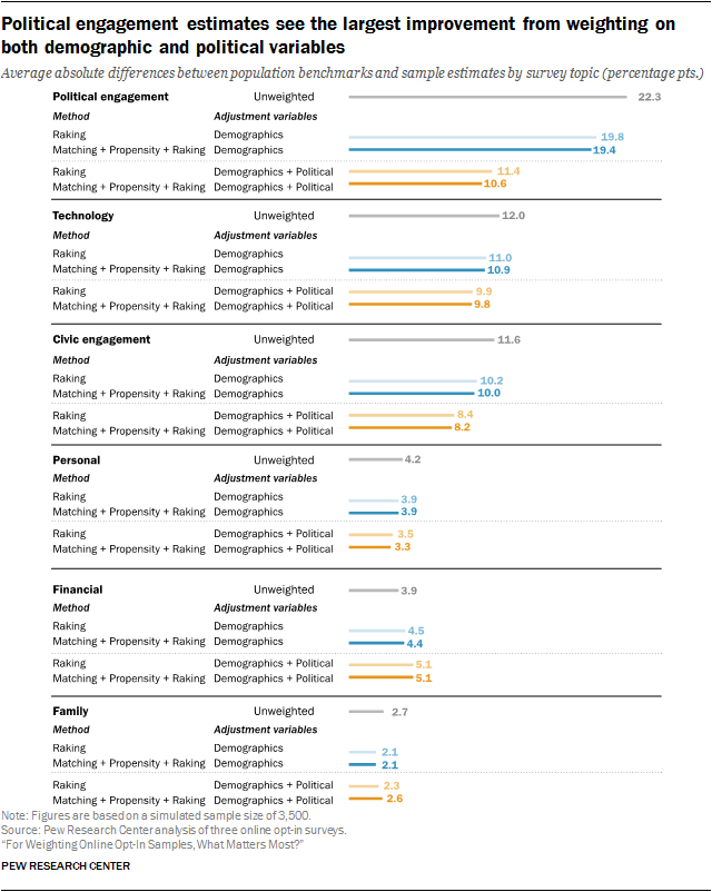
In terms of improving the accuracy of estimates, the results for individual survey topics (e.g., personal finances, technology, household characteristics) were similar to what was observed in the aggregate. Specifically, the study finds that the choice of adjustment variables mattered much more than the choice of statistical method. That said, the effect varied considerably from topic to topic.
The example comparing the least complex method, raking, to the more elaborate approach of matching followed by propensity adjustment and raking (“M+P+R”) across topics is illustrative of the general pattern. For the political engagement topic, M+P+R resulted in slightly lower bias than raking with both sets of adjustment variables, but the two methods were largely indistinguishable for the remaining topics. Meanwhile, the difference between adjusting on demographics alone and including additional political variables can be substantial. The difference was most dramatic for political engagement, which had an average bias of 22.3 percentage points unweighted – higher than any other topic. M+P+R with demographic variables reduced this by 2.9 points, but the inclusion of political variables reduced the average bias by an additional 8.8 points.
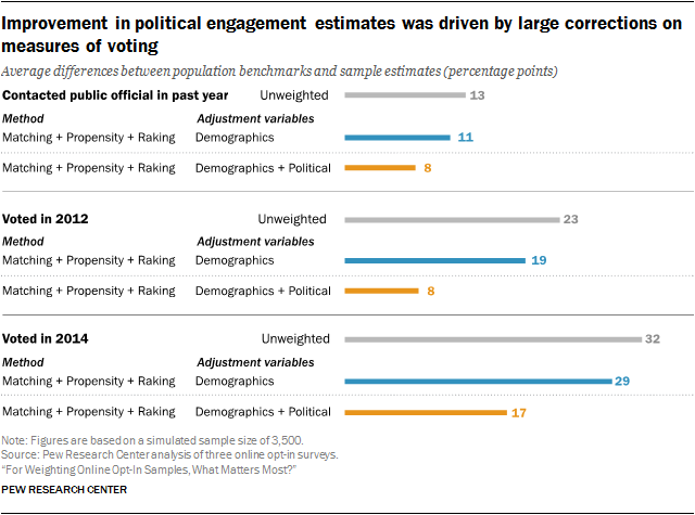
For political engagement benchmarks, the unweighted estimates substantially overrepresented adults who voted in 2014 and 2012 by 32 and 23 percentage points respectively. While M+P+R with demographic variables reduced these biases somewhat (by 3 and 4 points for the respective voting years), the inclusion of political variables in adjustment reduced the bias in the 2012 and 2014 votes by an additional 11 and 12 points respectively. This is likely due to the inclusion of voter registration as one of the political adjustment variables. Prior to weighting, registered voters were overrepresented by 19 percentage points, and it is natural that weighting registered voters down to their population proportion would also bring down the share who report having voted. The reduction in estimated bias on the share who reported contacting or visiting a public official in the past year makes intuitive sense as well, since it is plausible that those individuals are also more likely to be registered to vote.
However, even though the addition of political variables corrected a great deal of bias on these measures, large biases remained, with voting in 2012 overestimated by 8 points and voting in 2014 overestimated by 17 points. It is very possible that at least some of this remaining bias reflects individuals claiming to have voted when they did not, either because they forgot or because voting is socially desirable. Either way, the use of political variables in adjustment is not a silver bullet.
The effect of adjustment on questions about personal finances merits particular attention. On these questions, weighting caused the average estimated bias to increase rather than decrease, and the use of the expanded political variables made the increase even larger. Prior to any adjustment, the samples tend toward lower levels of economic well-being than the general public. For example, individuals with annual household incomes of $100,000 or more were underrepresented by about 8 percentage points, while those with incomes of under $20,000 were overrepresented by about 4 points. The share of respondents employed full-time was about 6 points lower than the population benchmark, while the percentage unemployed, laid off or looking for work was almost 5 points higher than among the population. The percentage who report that a member of their household has received food stamps in the past year was 13 points higher than the benchmark.
At the same time, respondents tended to have higher levels of education than the general public. The unweighted share with postgraduate degrees was 6 percentage points higher than the population value, and the percentage with less than a high school education 8 points lower.
Adjusting on core demographic variables corrected this educational imbalance and reduced the average education level of the survey samples. But in doing so, the average level of economic well-being was reduced even further, and biases on the financial measures were magnified rather than reduced. Because financial well-being and voter registration are also positively correlated, the inclusion of the expanded political variables produces even larger biases for these variables. This pattern suggests that weighting procedures could benefit from the inclusion of one or more additional variables that capture respondents’ economic situations more directly than education.
For benchmarks pertaining to civic engagement and technology, the reduction in bias from the inclusion of political variables was just over twice that of demographics alone, although in both cases the reductions were smaller than for political engagement. On the other hand, bias reduction for the personal and family topics was minimal for both sets of variables.
For some subgroups, more elaborate adjustments outperform raking
While there may be little to be gained from very large sample sizes or more complex statistical methods as far as general population estimates are concerned, there could be more pronounced differences between adjustment methods or more of an impact from increasing sample size for survey estimates based on population subgroups. In fact, an appealing feature of the machine-learning models used in matching and propensity weighting is the possibility that they will detect imbalances within subgroups that a researcher might not think to account for with raking.
For most subgroups, raking performed nearly as well as more elaborate approaches. However, there were a few subgroups that saw somewhat larger improvements in accuracy with more complex approaches. To minimize the number of moving parts in this particular analysis, these results are all based on a sample size of n=3,500 and on adjustments using both the demographic and political variables. Estimates based on college graduates had an average estimated bias of 6.5 percentage points with raking versus 5.5 points with a combination of matching, propensity weighting and raking. Similarly, average estimated bias on Hispanic estimates was 10.5 percentage points with raking versus 9.8 with the combination method. Similar, though smaller, differences were found for estimates based on adults ages 18-29, those ages 30-49, and men. Conversely, estimates for those with no more than a high school education were somewhat more accurate with raking. Estimates for other major demographic subgroups did not appear to be affected by the choice of statistical method.
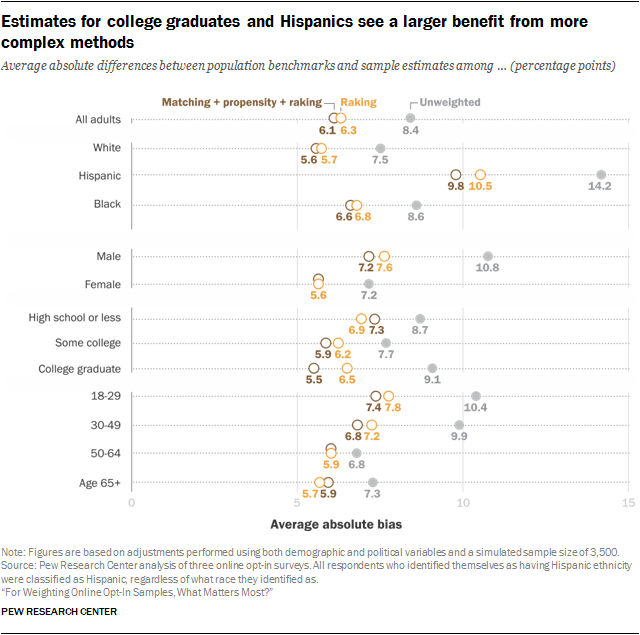
The pattern for Hispanics is particularly noteworthy. Estimates for this group had the largest average bias, both before weighting and after. The fact that M+P+R performed better than raking suggests that there are imbalances in the Hispanic composition that are not sufficiently captured by the raking specification. While this was the case for other groups as well (e.g., college graduates), Hispanics also saw much larger benefits from a larger starting sample size than other subgroups. At n=2,000, the average bias for Hispanic estimates was 10.2 percentage points. This steadily declined to 9 points at n=8,000 without leveling off, for a total change of 1.2 points. In comparison, the next-largest shifts were observed for college graduates, men, and adults younger than 30, at 0.4 points. This implies that even with 8,000 cases to choose from, the quality of Hispanic matches was poor and problematic in ways that subsequent propensity weighting and raking steps were unable to overcome. While all subgroups exhibited biases, the representation of Hispanics is particularly challenging and will require additional efforts that go well beyond those tested in this study.
For partisan measures, adding political variables to weighting adjustment can make online opt-in estimates more Republican
While benchmark comparisons provide an important measure of data quality, public opinion researchers are usually interested in studying attitudes and behaviors that lack the same kind of ground truth that can be used to gauge their accuracy. When gold-standard benchmarks are not available, one way to assess online opt-in polls is to look for alignment with probability-based polls conducted at roughly the same point in time. Although these polls are not without flaws of their own, well-designed and executed probability-based methods tend to be more accurate.20
In this study, there were several measures that could be compared to contemporaneous public polling: Barack Obama’s presidential approval, attitudes about the Affordable Care Act, and presidential vote preference in the 2016 election. These kinds of partisan measures are particularly relevant given that a previous Pew Research Center study found that online opt-in samples ranged from 3 to 8 percentage points more Democratic than comparable RDD telephone surveys.
The surveys used in this study showed a similar pattern. The synthetic population dataset had a distribution of 30% Democrat, 22% Republican and 48% independent or some other party, very close to the distribution found on the GSS and Pew Research Center surveys used in its creation. In comparison, with demographics-only raking, the opt-in samples used in this study were on average 4 points more Republican and 8 points more Democratic than the synthetic population dataset – more partisan in general, but disproportionately favoring Democrats. This is almost identical to the partisan distribution without any weighting at all.
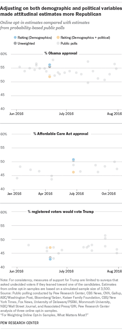
Using the political variables (which include party identification) in addition to demographics brings partisanship in line with the synthetic frame, reducing the share of Democrats more than the share of Republicans, and substantially increasing the share of independents.
This has a commensurate effect on public opinion measures that are associated with partisanship, moving them several points in the Republican direction. For example, when raking on demographics only, Obama’s approval rating was 56%, while adding political variables reduced this to 52%. Similarly, support for the Affordable Care Act dropped about 5 percentage points (from 51% to 46%) when the political variables were added to the raking adjustment. Support for Donald Trump among registered voters increased 4 points (from 43% to 47%) when the political variables were added.21
This raises the important question of whether these shifts in a Republican direction represent an improvement in data quality. The demographically weighted estimates do appear to be more Democratic than the probability-based polling with respect to each of these three measures, although in each case, they are not so different as to be entirely implausible. Although it is not possible to say definitively that the estimates that adjust on both demographic and political variables are more accurate, they do appear to be more in line with the trends observed in the other surveys.
While there appears to be a partisan tilt in many online opt-in surveys that should be addressed, particularly research focused on political topics, a great deal of caution is warranted. The partisan distribution of the American public changes over time, and the use of out-of-date weighting parameters could hide real changes in public opinion.
Less partisan, more ideological measures showed smaller changes when political variables were added to weighting
This study included a number of other attitudinal measures for which comparisons to other public polling was not possible. Nevertheless, it is still helpful to see the extent to which they are sensitive to decisions about weighting procedures. Many of these measures capture ideological but not necessarily partisan differences. Adjusting on both demographic and political variables tended to shift these measures in a more conservative direction, though the effect was both less pronounced and less consistent than for overtly partisan measures. For simplicity, the discussion is limited to estimates produced via raking, though as with the other attitudinal measures, there were no discernible differences from estimates employing more complex methods.
Using political variables in addition to demographics brought the percentage who said there is a lot of discrimination against blacks from 58% to 55%; against gays and lesbians, from 60% to 57%; and against Hispanics, from 52% to 49%. Support for marijuana legalization decreased from 61% to 58%.
The adjustment’s effects on other attitudinal estimates were more muted. The percentage who agreed with the statement “Immigrants today strengthen our country because of their hard work and talents” was essentially unchanged, going from 51% to 50%. The percentage who agreed that “Government should do more to solve problems” was 56% for demographics and 55% for demographics + political variables. The percentage who agreed with the statement “The economic system in this country unfairly favors powerful interests” stayed at 72%, regardless of whether only demographics or both demographics and political variables were used for adjustment. The share saying race relations in the United States were “getting better” went from 21% to 19%.
The study also contained questions about respondents’ engagement with public affairs and with the news. Adjusting on both demographic and political variables made these online opt-in estimates less engaged, with the percentage who would say they follow what’s going on in government and public affairs “most of the time” decreasing from 38% to 34% and the percentage who would say they follow the news “all or most of the time” falling from 48% to 44%. These somewhat larger shifts are in line with the reductions in political and civic engagement that were observed on benchmarks.


