
Historically, public opinion surveys have relied on the ability to adjust their datasets using a core set of demographics – sex, age, race and ethnicity, educational attainment, and geographic region – to correct any imbalances between the survey sample and the population. These are all variables that are correlated with a broad range of attitudes and behaviors of interest to survey researchers. Additionally, they are well measured on large, high-quality government surveys such as the American Community Survey (ACS), conducted by the U.S. Census Bureau, which means that reliable population benchmarks are readily available.
But are they sufficient for reducing selection bias6 in online opt-in surveys? Two studies that compared weighted and unweighted estimates from online opt-in samples found that in many instances, demographic weighting only minimally reduced bias, and in some cases actually made bias worse.7 In a previous Pew Research Center study comparing estimates from nine different online opt-in samples and the probability-based American Trends Panel, the sample that displayed the lowest average bias across 20 benchmarks (Sample I) used a number of variables in its weighting procedure that went beyond basic demographics, and it included factors such as frequency of internet use, voter registration, party identification and ideology.8 Sample I also employed a more complex statistical process involving three stages: matching followed by a propensity adjustment and finally raking (the techniques are described in detail below).
The present study builds on this prior research and attempts to determine the extent to which the inclusion of different adjustment variables or more sophisticated statistical techniques can improve the quality of estimates from online, opt-in survey samples. For this study, Pew Research Center fielded three large surveys, each with over 10,000 respondents, in June and July of 2016. The surveys each used the same questionnaire, but were fielded with different online, opt-in panel vendors. The vendors were each asked to produce samples with the same demographic distributions (also known as quotas) so that prior to weighting, they would have roughly comparable demographic compositions. The survey included questions on political and social attitudes, news consumption, and religion. It also included a variety of questions drawn from high-quality federal surveys that could be used either for benchmarking purposes or as adjustment variables. (See Appendix A for complete methodological details and Appendix F for the questionnaire.)
This study compares two sets of adjustment variables: core demographics (age, sex, educational attainment, race and Hispanic ethnicity, and census division) and a more expansive set of variables that includes both the core demographic variables and additional variables known to be associated with political attitudes and behaviors. These additional political variables include party identification, ideology, voter registration and identification as an evangelical Christian, and are intended to correct for the higher levels of civic and political engagement and Democratic leaning observed in the Center’s previous study.
The analysis compares three primary statistical methods for weighting survey data: raking, matching and propensity weighting. In addition to testing each method individually, we tested four techniques where these methods were applied in different combinations for a total of seven weighting methods:
- Raking
- Matching
- Propensity weighting
- Matching + Propensity weighting
- Matching + Raking
- Propensity weighting+ Raking
- Matching + Propensity weighting + Raking
Because different procedures may be more effective at larger or smaller sample sizes, we simulated survey samples of varying sizes. This was done by taking random subsamples of respondents from each of the three (n=10,000) datasets. The subsample sizes ranged from 2,000 to 8,000 in increments of 500.9 Each of the weighting methods was applied twice to each simulated survey dataset (subsample): once using only core demographic variables, and once using both demographic and political measures.10 Despite the use of different vendors, the effects of each weighting protocol were generally consistent across all three samples. Therefore, to simplify reporting, the results presented in this study are averaged across the three samples.
Often researchers would like to weight data using population targets that come from multiple sources. For instance, the American Community Survey (ACS), conducted by the U.S. Census Bureau, provides high-quality measures of demographics. The Current Population Survey (CPS) Voting and Registration Supplement provides high-quality measures of voter registration. No government surveys measure partisanship, ideology or religious affiliation, but they are measured on surveys such as the General Social Survey (GSS) or Pew Research Center’s Religious Landscape Study (RLS).
For some methods, such as raking, this does not present a problem, because they only require summary measures of the population distribution. But other techniques, such as matching or propensity weighting, require a case-level dataset that contains all of the adjustment variables. This is a problem if the variables come from different surveys.
To overcome this challenge, we created a “synthetic” population dataset that took data from the ACS and appended variables from other benchmark surveys (e.g., the CPS and RLS). In this context, “synthetic” means that some of the data came from statistical modeling (imputation) rather than directly from the survey participants’ answers.11
The first step in this process was to identify the variables that we wanted to append to the ACS, as well as any other questions that the different benchmark surveys had in common. Next, we took the data for these questions from the different benchmark datasets (e.g., the ACS and CPS) and combined them into one large file, with the cases, or interview records, from each survey literally stacked on top of each other. Some of the questions – such as age, sex, race or state – were available on all of the benchmark surveys, but others have large holes with missing data for cases that come from surveys where they were not asked.
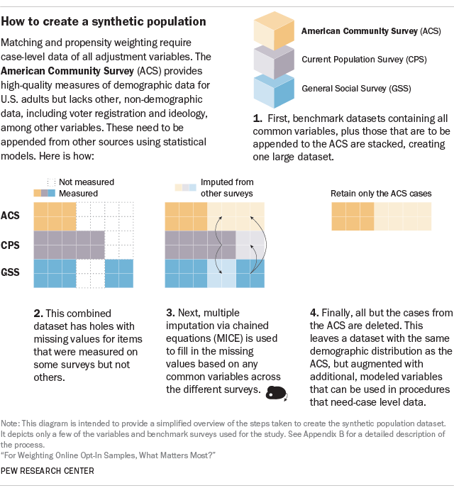
The next step was to statistically fill the holes of this large but incomplete dataset. For example, all the records from the ACS were missing voter registration, which that survey does not measure. We used a technique called multiple imputation by chained equations (MICE) to fill in such missing information.12 MICE fills in likely values based on a statistical model using the common variables. This process is repeated many times, with the model getting more accurate with each iteration. Eventually, all of the cases will have complete data for all of the variables used in the procedure, with the imputed variables following the same multivariate distribution as the surveys where they were actually measured.
The result is a large, case-level dataset that contains all the necessary adjustment variables. For this study, this dataset was then filtered down to only those cases from the ACS. This way, the demographic distribution exactly matches that of the ACS, and the other variables have the values that would be expected given that specific demographic distribution. We refer to this final dataset as the “synthetic population,” and it serves as a template or scale model of the total adult population.
This synthetic population dataset was used to perform the matching and the propensity weighting. It was also used as the source for the population distributions used in raking. This approach ensured that all of the weighted survey estimates in the study were based on the same population information. See Appendix B for complete details on the procedure.
Raking
For public opinion surveys, the most prevalent method for weighting is iterative proportional fitting, more commonly referred to as raking. With raking, a researcher chooses a set of variables where the population distribution is known, and the procedure iteratively adjusts the weight for each case until the sample distribution aligns with the population for those variables. For example, a researcher might specify that the sample should be 48% male and 52% female, and 40% with a high school education or less, 31% who have completed some college, and 29% college graduates. The process will adjust the weights so that gender ratio for the weighted survey sample matches the desired population distribution. Next, the weights are adjusted so that the education groups are in the correct proportion. If the adjustment for education pushes the sex distribution out of alignment, then the weights are adjusted again so that men and women are represented in the desired proportion. The process is repeated until the weighted distribution of all of the weighting variables matches their specified targets.
Raking is popular because it is relatively simple to implement, and it only requires knowing the marginal proportions for each variable used in weighting. That is, it is possible to weight on sex, age, education, race and geographic region separately without having to first know the population proportion for every combination of characteristics (e.g., the share that are male, 18- to 34-year-old, white college graduates living in the Midwest). Raking is the standard weighting method used by Pew Research Center and many other public pollsters.
In this study, the weighting variables were raked according to their marginal distributions, as well as by two-way cross-classifications for each pair of demographic variables (age, sex, race and ethnicity, education, and region).
Matching
Matching is another technique that has been proposed as a means of adjusting online opt-in samples. It involves starting with a sample of cases (i.e., survey interviews) that is representative of the population and contains all of the variables to be used in the adjustment. This “target” sample serves as a template for what a survey sample would look like if it was randomly selected from the population. In this study, the target samples were selected from our synthetic population dataset, but in practice they could come from other high-quality data sources containing the desired variables. Then, each case in the target sample is paired with the most similar case from the online opt-in sample. When the closest match has been found for all of the cases in the target sample, any unmatched cases from the online opt-in sample are discarded.
If all goes well, the remaining matched cases should be a set that closely resembles the target population. However, there is always a risk that there will be cases in the target sample with no good match in the survey data – instances where the most similar case has very little in common with the target. If there are many such cases, a matched sample may not look much like the target population in the end.
There are a variety of ways both to measure the similarity between individual cases and to perform the matching itself.13 The procedure employed here used a target sample of 1,500 cases that were randomly selected from the synthetic population dataset. To perform the matching, we temporarily combined the target sample and the online opt-in survey data into a single dataset. Next, we fit a statistical model that uses the adjustment variables (either demographics alone or demographics + political variables) to predict which cases in the combined dataset came from the target sample and which came from the survey data.
The kind of model used was a machine learning procedure called a random forest. Random forests can incorporate a large number of weighting variables and can find complicated relationships between adjustment variables that a researcher may not be aware of in advance. In addition to estimating the probability that each case belongs to either the target sample or the survey, random forests also produce a measure of the similarity between each case and every other case. The random forest similarity measure accounts for how many characteristics two cases have in common (e.g., gender, race and political party) and gives more weight to those variables that best distinguish between cases in the target sample and responses from the survey dataset.14
We used this similarity measure as the basis for matching.
The final matched sample is selected by sequentially matching each of the 1,500 cases in the target sample to the most similar case in the online opt-in survey dataset. Every subsequent match is restricted to those cases that have not been matched previously. Once the 1,500 best matches have been identified, the remaining survey cases are discarded.
For all of the sample sizes that we simulated for this study (n=2,000 to 8,000), we always matched down to a target sample of 1,500 cases. In simulations that started with a sample of 2,000 cases, 1,500 cases were matched and 500 were discarded. Similarly, for simulations starting with 8,000 cases, 6,500 were discarded. In practice, this would be very wasteful. However, in this case, it enabled us to hold the size of the final matched dataset constant and measure how the effectiveness of matching changes when a larger share of cases is discarded. The larger the starting sample, the more potential matches there are for each case in the target sample – and, hopefully, the lower the chances of poor-quality matches.
Propensity weighting
A key concept in probability-based sampling is that if survey respondents have different probabilities of selection, weighting each case by the inverse of its probability of selection removes any bias that might result from having different kinds of people represented in the wrong proportion. The same principle applies to online opt-in samples. The only difference is that for probability-based surveys, the selection probabilities are known from the sample design, while for opt-in surveys they are unknown and can only be estimated.
For this study, these probabilities were estimated by combining the online opt-in sample with the entire synthetic population dataset and fitting a statistical model to estimate the probability that a case comes from the synthetic population dataset or the online opt-in sample. As with matching, random forests were used to calculate these probabilities, but this can also be done with other kinds of models, such as logistic regression.15 Each online opt-in case was given a weight equal to the estimated probability that it came from the synthetic population divided by the estimated probability that it came from the online opt-in sample. Cases with a low probability of being from the online opt-in sample were underrepresented relative to their share of the population and received large weights. Cases with a high probability were overrepresented and received lower weights.
As with matching, the use of a random forest model should mean that interactions or complex relationships in the data are automatically detected and accounted for in the weights. However, unlike matching, none of the cases are thrown away. A potential disadvantage of the propensity approach is the possibility of highly variable weights, which can lead to greater variability for estimates (e.g., larger margins of error).
Combinations of adjustments
Some studies have found that a first stage of adjustment using matching or propensity weighting followed by a second stage of adjustment using raking can be more effective in reducing bias than any single method applied on its own.16 Neither matching nor propensity weighting will force the sample to exactly match the population on all dimensions, but the random forest models used to create these weights may pick up on relationships between the adjustment variables that raking would miss. Following up with raking may keep those relationships in place while bringing the sample fully into alignment with the population margins.
These procedures work by using the output from earlier stages as the input to later stages. For example, for matching followed by raking (M+R), raking is applied only the 1,500 matched cases. For matching followed by propensity weighting (M+P), the 1,500 matched cases are combined with the 1,500 records in the target sample. The propensity model is then fit to these 3,000 cases, and the resulting scores are used to create weights for the matched cases. When this is followed by a third stage of raking (M+P+R), the propensity weights are trimmed and then used as the starting point in the raking process. When first-stage propensity weights are followed by raking (P+R), the process is the same, with the propensity weights being trimmed and then fed into the raking procedure.


