
In addition to point estimates (e.g., % approving of President Barack Obama’s job performance), public opinion polls are often used to determine what factors explain a given attitude or behavior. For example, is education level or gender more predictive of Obama approval? This type of analysis involves testing the effects of multiple variables simultaneously. One possibility that researchers have discussed is that while some nonprobability samples may not provide very accurate point estimates, they might be able to provide accurate information about how different factors relate to one another (i.e., multivariate relationships).
To test this, we identified four outcomes (smoke daily, volunteered in past 12 months, always vote in local elections, and has health coverage) measured in all of the study samples, as well as in a high quality federal survey. By design, this set of outcomes includes variables that we know from the benchmarking were very difficult to estimate accurately (e.g., volunteering), as well as variables that were generally estimated accurately (e.g., health coverage). We also identified a set of explanatory variables common to these surveys: age, education, gender, race/ethnicity and region. For each sample, we estimated four regression models (one for each of the outcomes) using the same set of explanatory demographics. While these models are simplistic, they are consistent across the study samples.
With each of these models estimated, the key question was then, How well do these models, created using online samples, explain the actual behavior of a representative sample of U.S. adults? We used the microdataset for the federal survey as that representative sample. For each of the 40 models (10 samples, four outcomes), we took the coefficients from the nonprobability samples and the American Trends Panel (ATP) and applied them to responses in the federal dataset, generating a predicted value for the outcome. We then calculated the rate at which the models that were fit using nonprobability samples were able to correctly predict the true value for each respondent in the benchmark sample (% correctly classified).
Samples that performed relatively well in the benchmarking also performed relatively well in this analysis. Samples I, H and the ATP had the lowest average biases in the benchmarking analysis, and they yielded the regression estimates that were the most likely to correctly classify a randomly sampled, benchmark survey respondent on these four outcomes. As presented at the top of this report, the average share of the federal survey respondents classified correctly across the four outcomes is 76% for sample I, 74% for sample H and 72% for the ATP. The bottom of this ranking is also highly consistent with the benchmarking. The three samples showing the largest average errors in the benchmarking (C, A and D) yielded the regression estimates that are the least likely to correctly classify a randomly sampled adult on these four outcomes. The average percentage classified correctly is 69% for sample C and 66% each for samples A and D.
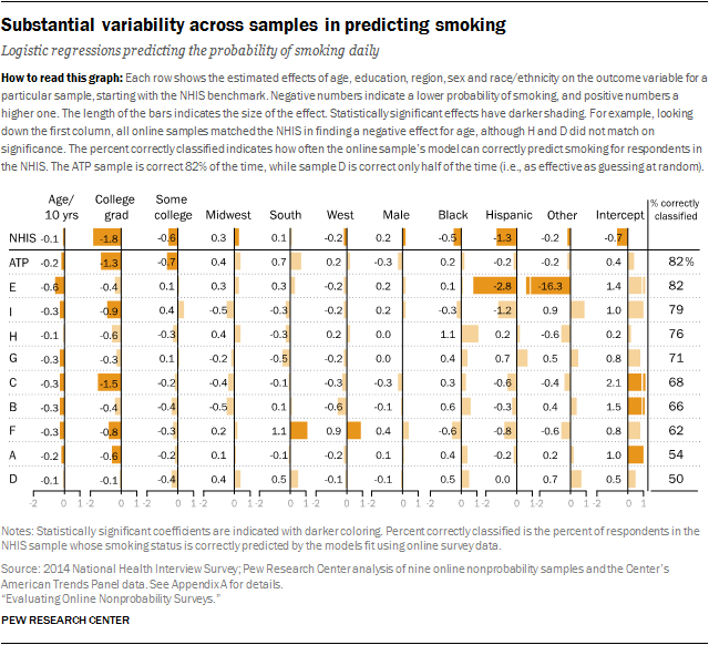
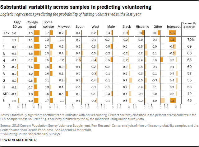
Looked at individually, the four outcomes vary considerably in the extent to which they differentiate among the samples. For daily smoking, the percentage of federal survey respondents correctly classified was 82% for the best models and 50% for the worst. Similarly, for the volunteering measure, the share of federal survey respondents correctly classified was 70% for the best model and 46% for the worst. For both of these outcomes, the samples that were most accurate on the point estimates also exhibited the most predictive accuracy in the regressions. The reverse was also true: Samples with the least accurate point estimates were also least accurate in the regressions. This demonstrates that the assumption that multivariate relationships will be accurate even when point estimates are not does not hold up.
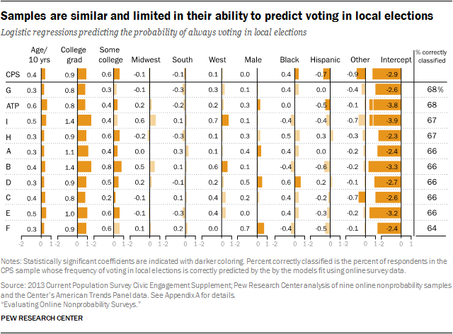
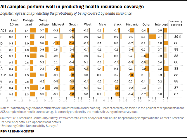
For health coverage, all of the samples were relatively close to the benchmark, and all display similarly high levels of predictive accuracy, with the best and worst models differing by only 2 percentage points (89% vs. 87%). The voting models also yielded a narrow range in the percent correctly classified (64% to 68%), but the overall level of accuracy was lower.
Marginal effects associated with race and ethnicity are rarely correct
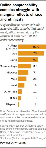
Substantively, the conclusions one would draw from the coefficients of these regression models using the nonprobability samples would likely differ from the conclusions drawn using the benchmark survey. While the nonprobability samples often succeed in capturing the effects associated with education and age, they rarely capture the effects associated with race and ethnicity that one finds in the benchmark surveys.
For example, according to the NHIS model estimates, daily smoking is negatively associated with age, education, Hispanic ethnicity and being black. For the most part, the nonprobability sample models show significant, negative effects for age and education. Only one of the nine nonprobability samples, however, has significant negative effects for both Hispanic ethnicity and black race.
This general pattern is seen in models for all four outcomes. We can quantify the pattern by leveraging the fact that, for each category, we have 36 nonprobability sample estimates (four outcomes modeled separately with nine samples). We noted whether each of those 36 estimated effects was consistent with the same effect estimated from the benchmark dataset with respect to direction and significance. If the estimated effect in the benchmark survey was nonsignificant, then the nonprobability effect estimate was coded as “correct” if and only if it was also nonsignificant, regardless of direction. If, by contrast, the estimated effect in the benchmark survey was statistically significant, then the nonprobability effect was coded as “correct” if and only if it was also statistically significant and in the same direction.
By this measure, the nonprobability samples “correctly” estimated the effect of being a college graduate 86% of the time (31 of 36 estimates) and “correctly” estimated the effect of age 78% of the time (28 of 36 estimates). These successes are no doubt related to the fact that age and education truly have strong associations with the four outcomes used in this analysis.
The nonprobability samples did not fare nearly as well in estimating the marginal effects from race and ethnicity. Based on the benchmark survey data, each of the four models show statistically significant effects for both Hispanic ethnicity and black race. Across the 36 nonprobability sample estimates, the Hispanic effect was “correct” only once (sample E on daily smoking). The effect associated with being black was “correct” only 8% of the time (once each for samples B, D and F). These results indicate that researchers using online nonprobability samples are at risk of drawing erroneous conclusions about the effects associated with race and ethnicity.
In other analyses presented in this report, focusing on the collective performance of the nonprobability samples tells, at best, only part of the discernable story about data quality. This particular analysis is different, however, because all of the nonprobability samples tend to estimate the marginal effects from age and education reasonably well and estimate the marginal effects from race and ethnicity poorly. Notably, sample I, which stands out as a top performer on several other metrics, looks unremarkable here.
By this standard, the results for the American Trends Panel are fairly similar to those from the nonprobability samples, but the ATP was more successful in capturing the marginal effect associated with Hispanic ethnicity. The ATP’s estimated Hispanicity effect was accurate for both health coverage and voting in local elections. This result is likely related to the fact that the ATP features Spanish-language as well as English administration, whereas the nonprobability samples were English only. The ATP also has a sample size advantage relative to the nonprobability samples. Each of the nonprobability samples features about n=1,000 interviews, whereas the average ATP sample size was roughly n=2,800, making it easier to detect a statistically significant difference. To test whether the ATP results are explained by the larger sample size, we replicated these regressions on 15 random subsamples of 1,000 ATP respondents and found that the conclusions were not substantively affected.


