
(Related posts: 5 things to keep in mind when you hear about Gen Z, Millennials, Boomers and other generations and How Pew Research Center will report on generations moving forward)
Opinions often differ by generation in the United States. For example, Gen Zers and Millennials are more likely than older generations to want the government to do more to solve problems, according to a January 2020 Pew Research Center survey. But will Gen Zers and Millennials always feel that way, or might their views on government become more conservative as they age? In other words, are their attitudes an enduring trait specific to their generation, or do they simply reflect a stage in life?
That question cannot be answered with a single survey. Instead, researchers need two things: 1) survey data collected over many years – ideally at least 50 years, or long enough for multiple generations to advance through the same life stages; and 2) a statistical tool called age-period-cohort (APC) analysis.
In this piece, we’ll demonstrate how to conduct age-period-cohort analysis to determine the effects of generation, using nearly 60 years of data from the U.S. Census Bureau’s Current Population Survey. Specifically, we’ll revisit two previous Center analyses that looked at generational differences in marriage rates and the likelihood of having moved residences in the past year to see how they hold up when we use APC analysis.
What is age-period-cohort analysis?
In a typical survey wave, respondents’ generation and age are perfectly correlated with each other. The two cannot be disentangled. Separating the influence of generation and life cycle requires us to have many years of data.
If we have data not just from 2020, but also from 2000, 1980 and earlier decades, we can compare the attitudes of different generations while they were passing through the same stages in the life cycle. For example, we can contrast a 25-year-old respondent in 2020 (who would be a Millennial) with a 25-year-old in 2000 (a Gen Xer) and a 25-year-old in 1980 (a Baby Boomer).
A dataset compiled over many years allows age and generation to be examined separately using age-period-cohort analysis. In this context, “age” denotes a person’s stage in the life cycle, “period” refers to when the data was collected, and “cohort” refers to a group of people who were born within the same time period. For this analysis, the cohorts we are interested in are generations – Generation Z, Millennials, Generation X and so on.
APC analysis seeks to parse the effects of age, period and cohort on a phenomenon. In a strictly mathematical sense, this is a problem because any one of those things can be exactly calculated from the other two (e.g., if someone was 50 years old in 2016, then we also know they were born circa 1966 because 2016 – 50 = 1966). If we only have data collected at one point in time, it’s not possible to identify conclusively whether apparent differences between generations are not just due to how old the respondents were when the data was collected. For example, we don’t know whether Millennials’ lower marriage rate in 2016 is a generational difference or simply a result of the fact that people ages 23 to 38 are less likely to be married, regardless of when they were born. Even if we have data from many years, any apparent trends could also be due to other factors that apply to all generations and age groups equally. We might mistakenly attribute a finding to age or cohort when it really should be attributed to period. This is called the “identification problem.” Approaches to APC analysis are all about getting around the identification problem in some way.
Using multilevel modeling for age-period-cohort analysis
A common approach for APC analysis is multilevel modeling. A multilevel model is a kind of regression model that can be fit to data that is structured in “groups,” which themselves can be units of analysis.
A classic example of multilevel modeling is in education research, where a researcher might have data on students from many schools. In this example, the two levels in the data are students and the schools they attend. Traits on both the student level (e.g., grade-point average, test scores) and the school level (e.g., funding, class size) could be important to understanding outcomes.
In APC analysis, things are a little different. In a dataset collected over many years, we can think of each respondent as belonging to two different but overlapping groups. The first is their generation, as determined by the year in which they were born. The second is the year in which the data was collected.
Fitting a multilevel model with groups for generation and year lets us isolate differences between cohorts (generations) and periods (years) while holding individual characteristics like age, sex and race constant. Placing period and cohort on a different level from age addresses the identification problem by allowing us to model all of these variables simultaneously.
Conducting age-period-cohort analysis with the Current Population Survey
One excellent resource that can support APC analysis is the Current Population Survey’s Annual Social and Economic Supplement (ASEC), conducted almost every year from 1962 to 2021. We’ll use data from the ASEC to address two questions:
- Does the lower marriage rate among today’s young adults reflect a generational effect, or is it explained by other factors?
- Does the relatively low rate of moving among today’s young adults reflect a generational effect, or is it explained by other factors?
In previous Center analyses, we held only age constant. This time, we want to separate generation not just from age, but also from period, race, gender and education.
Getting started
The data we’ll use in this analysis can be accessed through the Integrated Public Use Microdata Series (IPUMS). After selecting the datasets and variables you need, download the data (as a dat.gz file) and the XML file that describes the data and put them in the same folder. Then, use the package ipumsr to read the data in as follows:
library(tidyverse)
library(ipumsr)
asec_ddi <- read_ipums_ddi(ddi_file = "path/to/data/here.xml")
asec_micro <- read_ipums_micro(asec_ddi)
Next, process and clean the data. First, filter the data so it only includes adults (people ages 18 and older), and then create clean versions of the variables that will be in the model.
Here’s a look at the cleaning and filtering code we used. We coded anyone older than 80 as being 80 because the ASEC already coded them that way for some years. We applied that rule to every year in order to ensure consistency. We only created White, Black and Other categories for race because categories such as Hispanic and Asian weren’t measured until later. Finally, there were several years when the ASEC did not measure whether people moved residences in the past year, so we excluded those years from our analysis.
asec_rec <- asec_micro %>%
  # Filter to adults ages 18 or older
  filter(AGE >= 18) %>%

  # EDUC is completely missing for 1963 so exclude that year
  filter(YEAR != 1963) %>%

  # Drop an additional 8 cases for which education is coded as unknown
  filter(EDUC != 999) %>%

  # Remove a few hundred cases with weights less than or equal to 0
  filter(ASECWT > 0) %>%

  # Recode variables for analysis
  mutate(SEX = as_factor(SEX) %>% fct_drop(),

         EDUCCAT = case_when(EDUC < 80 ~ "HS or less",
                             EDUC >= 80 & EDUC <= 110 ~ "Some coll",
                             EDUC > 110 & EDUC < 999 ~ "Coll grad",
                             EDUC == 999 ~ NA_character_) %>%
           as_factor(),

         # Age was topcoded at 90 from 1988-2001, then at 80 in 2002
         # and 2003, then at 85 from 2004-present. Since we're trying
         # to use the entire dataset, age will be topcoded at 80
         # across the board.
         AGE_TOPCODED = case_when(AGE >= 80 ~ 80,
                                  TRUE ~ as.numeric(AGE)),

         # White and Black are present for every single year, whereas
         # categories like Hispanic and Asian weren't added until
         # later.
         RACE_COLLAPSED = case_when(RACE == 100 ~ "White",
                                    RACE == 200 ~ "Black",
                                    TRUE ~ "Other") %>%
           as_factor(),

         # Calculate birth year from age and survey year
         YEAR_BORN = YEAR - AGE_TOPCODED,

         # Calculate generation from birth year
         GENERATION = case_when(YEAR_BORN <= 1945 ~
                                  "Silent and older",
                                YEAR_BORN %in% 1946:1964 ~ "Boomer",
                                YEAR_BORN %in% 1965:1980 ~ "Xer",
                                YEAR_BORN %in% 1981:1996 ~
                                  "Millennial",
                                YEAR_BORN >= 1997 ~ "Gen Z") %>%
           as_factor(),

         # Create binary indicators for outcome variables
         MARRIED = case_when(MARST %in% 1:2 ~ 1,
                             TRUE ~ 0),

         # Note that MIGRATE1 is missing for the years 1962,
         # 1972-1975, 1977-1980, and 1985. The documentation also
         # indicates that the 1995 data seem unusual.
         MOVED1YR = case_when(MIGRATE1 %in% 3:5 ~ 1,
                              is.na(MIGRATE1) ~ NA_real_,
                              TRUE ~ 0)) %>%

  # Group by YEAR and the household ID to calculate the number of
  # adults in each respondent's household
  group_by(YEAR, SERIAL) %>%
  mutate(ADULTS = n()) %>%
  ungroup() %>%

  # Retain only the variables we need for this analysis
  select(YEAR, SERIAL, PERNUM, ASECWT, AGE, AGE_TOPCODED, YEAR_BORN,
         GENERATION, SEX, EDUCCAT, RACE_COLLAPSED, MARRIED, MOVED1YR,
         ADULTS)
The full ASEC dataset has more than 6.7 million observations, with around 60,000 to 100,000 cases from each year. Without the computing power to fit a model to the entire dataset in any reasonable amount of time, one option is to sample a smaller number of cases per year, such as 2,000. To ensure that the sampled cases are still representative, sample them proportionally to their survey weight.
set.seed(20220617)
asec_rec_samp <- asec_rec %>%
  group_by(YEAR) %>%
  slice_sample(n = 1000, weight_by = ASECWT)
Model fitting
Now that the data has been processed, it’s ready for model fitting. This example uses the rstanarm package to fit the model using Bayesian inference.
Below, we fit a multilevel logistic regression model with marriage as the outcome variable; with age, number of adults in the household, sex, race and education as individual-level explanatory variables; and with period and generation as normally distributed random effects that shift the intercept depending on which groups an individual is in.
library(rstanarm)
fit_marriage <- stan_glmer(MARRIED ~ AGE_TOPCODED + I(AGE_TOPCODED^2)
                           + ADULTS + SEX + RACE_COLLAPSED + EDUCCAT +
                             (1 | YEAR) + (1 | GENERATION),
                           data = asec_rec_samp,
                           family = binomial(link = "logit"),
                           chains = 4,
                           iter = 1000,
                           cores = 4,
                           refresh = 1,
                           adapt_delta = 0.97,
                           QR = TRUE)
Regression models are largely made up of two components: the outcome variable and some explanatory variables. Characteristics that are measured on each individual in the data and that could be related to the outcome variable are potentially good explanatory variables. Every model also contains residual error, which captures anything that influences the outcome variable other than the explanatory variables; this can be thought of as encompassing unique qualities that make all individuals in the data different from one another. A multilevel regression model will also capture unique qualities that make each group in the data different from one another. The model may optionally include group-level explanatory variables as well.
The groups don’t need to be neatly nested within one another, allowing for flexibility in the kinds of situations to which multilevel modeling can apply. In our example, we model age as a continuous, individual-level predictor while modeling generation (cohort) and period as groups that each have different, discrete effects on the outcome variable. Separating age from period and cohort by placing them on different levels allows us to model all of them without running head-on into the identification problem. However, this is premised on a number of important assumptions that may not always hold up in practice.
By modeling the data like this, we are treating the relationship between period or generation and marriage rates as discrete, where each period or generation has its own distinct relationship. If there is a smooth trend over time, the model does not estimate the trend itself, instead looking at each period or generation in isolation. We are, however, modeling age as a continuous trend.
Separating generation from other factors
Our research questions above concern whether the differences by generation that show up in the data can still be attributed to generation after controlling for age, cohort and other explanatory variables.
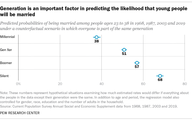
In a report on Millennials and family life, Pew Research Center looked at ASEC’s data on people who were 23 to 38 years old in four specific years – 2019, 2003, 1987 and 1968. Each of these groups carried a generation label – Millennial, Gen X, Boomer and Silent – and the report noted that younger generations were less likely to be married than older ones.
Now that we have a model, we can reexamine this conclusion, decoupling generation from age and period. The model can return predicted probabilities of being married for any combination of variables passed to it, including combinations that didn’t previously exist in the data – and combinations that are, by definition, impossible. The model can, for example, predict how likely it is that a Millennial who was between ages 23 and 38 in 1968 would be married, even if no such person can exist. That’s useful not for what it represents in and of itself, but for what it can explain about the influence of generation on getting married.
In order to create predicted probabilities, the first requirement is to create a dataset on which the model will predict probabilities. This dataset should have every variable used in the model.
Here, we create a function that takes five inputs: the model, the original data, a generation category (cohorts), a range of years (periods) and a range of ages. This function will take everybody in the ASEC data for the given years and ages (regardless of whether they were in the subset used to fit the model) and set all their generations to be the same while keeping everything else unchanged, whether the resulting input makes sense in real life or not. This simulated ASEC data is then passed to the posterior_predict() function from rstanarm, which gives us a 2,000-by-n matrix, where n is the number of observations in the new data passed to it. We then compute the weighted mean of the predicted probabilities across the observations, giving us 2,000 weighted means. These 2,000 weighted means represent draws from a distribution estimating the predicted probability. We summarize this distribution by taking its median, as well as the 2.5th and 97.5th percentiles to create a 95% interval to express uncertainty.
We then run this function four times, once for each generation, on everyone in the ASEC data who was ages 23 to 38 during each of the four years we studied in the report. First, the function estimates the marriage rate among those people if, hypothetically, they were all Millennials, regardless of what year they appear in the ASEC data. Next, it estimates the marriage rate among those same people if, hypothetically, they were all Gen Xers. Then the function estimates the marriage rate if they were all Boomers or members of the Silent Generation, respectively.
# Helper function to get estimates for hypothetical scenarios
estimate_hypothetical <- function(fit, df, generation, seed) {

  # Set generation to the same value for all cases
  df$GENERATION <- factor(generation)

  # Get means for each
  ppreds <- posterior_predict(fit, newdata = df, seed = seed)
  pmeans <- apply(ppreds, MARGIN = 1, weighted.mean, w = df$ASECWT)

  # Get median and 95% intervals for the posterior mean
  estimate <- quantile(pmeans, probs = c(0.025, 0.5, 0.975)) %>%
    set_names("lower95", "median", "upper95")

  return(estimate)
}


# Filter to the years and age ranges from the original analysis
analysis_subset_marriage <- asec_rec %>%
  filter(YEAR %in% c(2019, 2003, 1987, 1968),
         AGE %in% 23:38)

# Get estimates for each generation
estimates_marriage <- c("Millennial", "Xer", "Boomer", "Silent and older") %>%
  set_names() %>%
  map_dfr(~estimate_hypothetical(fit = fit_marriage,
                                df = analysis_subset_marriage,
                                generation = .x,
                                seed = 20220907),
          .id = "GENERATION")
In statistical terms, we are drawing from the “posterior predictive distribution.” This allows us to generate estimates for hypothetical scenarios in which we manipulate generation while holding age, period and all other individual characteristics constant. While this is not anything that could ever happen in the real world, it’s a convenient and interpretable way to visualize how changing one predictor would affect the outcome (marriage rate).
Determining the role of generation
To answer the first of our research questions, let’s plot our predicted probabilities of being married. If we took all these people at each of these points in time and magically imbued them with everything that is unique to being a Millennial, the model estimates that 38% of them would be married. In contrast, if you imbued everyone with the essence of the Silent Generation, that estimate would be 68%. The numbers themselves aren’t important, as they don’t describe an actual population. Instead, we’re mainly interested in how different the numbers are from one another. In this case, the intervals do not overlap at all between the generations and there is a clear downward trend in the marriage rate. This is what we would expect to see if the lower marriage rate among Millennials reflects generational change that is not explained by the life cycle (age) or by other variables in the model (gender, race, education).
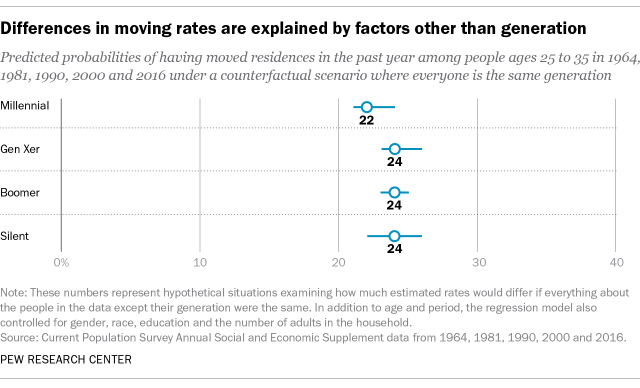
What about our second question about generational differences in the likelihood of having moved residences in the past year? The Center previously reported that Millennials were less likely to move than prior generations of young adults. That analysis was based on a similar approach that considered people who were ages 25 to 35 in 2016, 2000, 1990, 1981 and 1963, and identified them as Millennials, Gen Xers, “Late Boomers,” “Early Boomers” and Silents.
Using the ASEC dataset described above, we reexamined this pattern using age-period-cohort analysis. We fit the same kind of multilevel model to this outcome and plotted the predicted probabilities in the same way. In this case, there are no clear differences or trend across the generations, with overlapping intervals for the estimated share who moved in the past year. This suggests that the apparent differences between the generations are better explained by other factors in the model, not generation.
Conclusion
These twin analyses of marriage rates and moving rates illustrates several key points in generational research.
In some cases (e.g., moving), what looks like a generation effect is actually explained by other factors, such as race or education. In other cases (e.g., marriage), there is evidence of an enduring effect associated with one’s generation.
APC analysis requires an extended time series of data; a theory for why generation may matter; a careful statistical approach; and an understanding of the underlying assumptions being made.
