

(Related post: How to analyze Pew Research Center survey data in R)
Last year, I wrote an introductory blog post about how to access and analyze Pew Research Center survey data with R, a free, open-source software for statistical analysis. The post showed how to perform tasks using the survey package.
The survey package is ideal if you’re analyzing survey data and need variance estimates that account for complex sample designs, such as cluster samples or stratification. However, the first step of any data analysis is often exploring the data with simple but powerful summaries, such as crosstabs and plots. This usually requires significant re-coding of variables as well as data cleaning and other manipulation tasks that can be difficult and counterintuitive. Fortunately, something called the “tidyverse” is here to help.
In this post, I’ll show how to use tidyverse tools to do exploratory analyses of Pew Research Center survey data. (These tools, however, can be used with data from any source.)
What is the “tidyverse”?
R has a large community of users, many of whom make their own code freely available to other R users in the form of packages that implement specialized kinds of analyses or enable other programming tasks.
R packages are typically hosted on The Comprehensive R Archive Network (CRAN), but are also available on other primarily open-source code repositories like github, gitlab or bioconductor. One of the nice things about R is that anyone can build a package and contribute to the software’s development. But with so many packages (there were 14,366 on CRAN as of June 12, 2019), there are often many different ways to tackle the same challenge. This can lead to inconsistencies that are often confusing, making it harder on new users or those looking to develop their R skills.
Enter the tidyverse, a collection of R packages designed for data science that share a consistent design philosophy and produce code that can be more easily understood and shared. The tidyverse has a growing community of users, contributors and developers that aim to help R users access and learn these free, open-source tools. The book R for Data Science by Hadley Wickham and Garrett Grolemund walks through many key components of how to use these tools to do data science in R and can be accessed online for free.
Packages
For this post, we’ll need the tidyverse and haven packages. The haven package is the tidyverse’s solution for importing and exporting data from several different formats, including SPSS (the format in which most Center datasets are currently released), SAS and Stata.
The only functions from the haven package we’ll use here are read_sav() and as_factor(). All other functions referenced in this post come from packages like dplyr, forcats or ggplot2, which are loaded automatically with the tidyversepackage.
If you don’t already have these packages, you’ll need to install them in order to run the code in this post. Even if you have already installed them, you can update them by running the below code:
install.packages("tidyverse")
install.packages("haven")
Next, load the packages in with the library() function:
library(tidyverse)
#loads all "core" tidyverse packages like
#dplyr, tidyr, forcats, and ggplot2
library(haven)
Pipes
One of the most appealing features of the tidyverse is its emphasis on making code easier to read and understand. A key tool for improving the readability of tidyverse code is the pipe, a set of three characters that looks like this: %>%. Placing a pipe to the right of an object (such as data %>%) tells R to take the object on its left and send it to its right. This allows you to chain multiple commands together without getting lost in a hailstorm of parentheses.
Let’s use a pop culture dataset to illustrate this point. The starwars dataset that comes with the tidyverse package contains information on the characters from the movies, made available through the Star Wars API. Suppose we want to filter the dataset to all characters for whom a height is known, arrange the dataset in order of decreasing height and then change the height variable from centimeters to inches.
Here is the code to do this without using pipes:
mutate(arrange(filter(starwars, !is.na(height)), desc(height)), height = 0.393701 * height)And here’s the code with the pipe:
starwars %>%
filter(!is.na(height)) %>%
arrange(desc(height)) %>%
mutate(height = 0.393701 * height)
As far as R is concerned, these two pieces of code do exactly the same thing. But using a series of pipes makes it much easier for humans to read and understand exactly what’s going on, and in what order. The code above can be easily read as a series of steps: take the starwars dataset, filter it to cases where height is not missing, arrange the remaining cases by height in descending order, and, finally, change the height variable to inches.
Readability makes it easier to share your code with other people. Even if you’ll never share your code with anyone else, this approach will make it easier for you to understand your own code if you ever need to revisit it weeks, months or even years later when the details are no longer fresh in your memory. (This can also help you or your team avoid technical debt.)
Beyond readability, pipes make your code easier to maintain. It’s easy to remove a step, insert a new step or change the order when all of the commands are in a sequential series of pipes, rather than nested.
Loading the data into R
Let’s shift gears and return our attention to using tidyverse tools to analyze Pew Research Center survey data. You can download the Center’s datasets via this link, and you can learn more here about the kind of data we release and how to access it.
For the purposes of this backgrounder, we’ll use data from our April 2017 Political survey. We’ll walk through how to use tidyverse tools to calculate weighted survey estimates (specifically, approval of President Donald Trump) broken out by other variables in our dataset (education, race/ethnicity and generation).
The first step is to load the dataset into your R environment. Almost all of the datasets available to download from the Center are stored as .sav (SPSS) files. The haven package can import datasets created by SPSS and a number other programs such as Stata and SAS.
There are a few features of SPSS datasets that require special handling when loading data into R. SPSS files often contain variables with both character labels and numeric codes that are not necessarily sequential (e.g. for party ID, 1 = Republican, 2 = Democrat, 9 = Refused). SPSS also allows variables to have multiple, user-defined missing values. This sort of variable metadata is helpful, but it doesn’t quite align with any of R’s standard data types.
The haven package handles these differences by importing variables in a custom format called "labelled" and leaving the user to decide which of the numeric codes or value labels he or she wants to work with in R.
We’ll import the data using haven’s read_sav() function. We’ll set user_na = TRUE to ensure that responses such as “Don’t know” or “Refused” aren’t automatically converted to missing values. In this case, we also want to convert any labelled variables into factors so that we can work with value labels instead of the numeric codes (e.g. “Republican” instead of “1”). We do this by piping (%>%) the entire dataset to haven’s as_factor() function which converts any labelled variables in the dataset to factors.
Apr17 <- read_sav("Apr17 public.sav",
user_na = TRUE) %>%
as_factor()
Adding variables with mutate
The first question (q1) on the April 2017 survey asked whether or not respondents approved of Trump’s performance as president so far. The next question (q1a) asked respondents how strongly they approved or disapproved (“Very strongly,” “Not so strongly,” “Don’t know/Refused (VOL.)”). We want to use these two variables to create a new variable that combines q1 and q1a. This sort of re-coding is extremely common when working with survey data, but it can be a surprisingly difficult task when using only base R functions. The dplyrpackage, which is loaded automatically as part of the tidyverse package, includes a number of tools that make these sorts of data processing tasks much easier.
The most general of these is the mutate() function, which either adds new variables to a data frame or modifies existing variables. We’ll use mutate() in the code below to create a variable called trump_approval. The actual re-coding is done with the case_when() function, which evaluates a series of conditions and returns the value associated with the first one that applies.
Apr17 <- Apr17 %>%
mutate(trump_approval = case_when(

q1 == "Approve" & q1a == "Very strongly" ~ "Strongly approve",
q1 == "Approve" & q1a != "Very strongly" ~ "Not strongly approve",
q1 == "Disapprove" & q1a == "Very strongly" ~ "Strongly disapprove",
q1 == "Disapprove" & q1a != "Very strongly" ~ "Not strongly disapprove",
q1 == "Don't know/Refused (VOL.)" |
q1a == "Don't know/Refused (VOL.)" ~ "Refused"
) #this parentheses closes call to
#case_when and sends it to
#fct_relevel with %>%
%>%
fct_relevel("Strongly approve",
"Not strongly approve",
"Not strongly disapprove",
"Strongly disapprove",
"Refused"
) #this parentheses closes our call to fct_relevel
) #this parentheses closes our call to mutate
We supply a series of formulas to the case_when() function. Each formula is an “if-then” statement, where the left side (everything to the left of ~) describes a logical condition and the right side provides the value to return if that condition is true. As a reminder, you can type ?case_when() to access the help page (this works for any function in R, not just case_when()).
The first line of the call to case_when() is: q1 == "Approve" & q1a == "Very strongly" ~ "Strongly approve". This can be read to mean that respondent said “Approve” to q1 and answered “Very strongly” to q1a, so we’ll code them as “Strongly approve” in our new trump_approval variable. We use five different clauses to make these new categories and add the trump_approval variable to our dataset.
Because case_when() returns character variables when used this way, the last step is to pipe the variable to fct_relevel() from the forcats package. This converts trump_approval to a factor and orders the categories from “Strongly approve” to “Refused.”
We can run the table command on our new variable to verify that everything worked as intended.
table(Apr17$trump_approval, Apr17$q1)
##
##                  Approve      Disapprove              Don't know/
##                                                    Refused (VOL.)
##Strongly approve          476          0                         0
##Not strongly approve      130          0                         0
##Not strongly disapprove     0        143                         0
##Strongly disapprove         0        676                         0
##Refused                     0          0                        76
Having created our new trump_approval variable, we’d like to see how it breaks down according to a few different demographic characteristics: educational attainment (educ2 in the Apr17 dataset), race/ethnicty (racethn) and generation (gen5).
But educ2 has nine categories, some of which don’t have very many respondents. We thus want to collapse them into fewer categories with larger numbers of respondents. We can do this with the forcats function fct_collapse(). We use mutate() again to make new variables.
Let’s first check the answer options of educ2 to see the categories we need to collapse. Since we used as_factor() when we read the dataset in, educ2 is a factor variable. So, we can see the answer options by using the levels()function.
levels(Apr17$educ2)

## [1] "Less than high school (Grades 1-8 or no formal schooling)"
## [2] "High school incomplete (Grades 9-11 or Grade 12 with NO diploma)"
## [3] "High school graduate (Grade 12 with diploma or GED certificate)"
## [4] "Some college, no degree (includes some community college)"
## [5] "Two year associate degree from a college or university"
## [6] "Four year college or university degree/Bachelor's degree (e.g., BS, BA, AB)"
## [7] "Some postgraduate or professional schooling, no postgraduate degree"
## [8] "Postgraduate or professional degree, including master's, doctorate, medical or law degree"
## [9] "Don't know/Refused (VOL.)"
Now that we know the levels, we can collapse them into fewer categories. The first argument to fct_collapse() is the variable whose categories you want to collapse, in our case educ2. We assign new categories on the left, like “High school grad or less”, in the below example. We use the c() function to tell fct_collapse() these categories belong in our new “High school grad or less” category. Note that you need to use the exact names of these categories.
Apr17 <- Apr17 %>%
mutate(educ_cat = fct_collapse(educ2,
"High school grad or less" = c(
"Less than high school (Grades 1-8 or no formal schooling)",
"High school incomplete (Grades 9-11 or Grade 12 with NO diploma)",
"High school graduate (Grade 12 with diploma or GED certificate)"
),
"Some college" = c(
"Some college, no degree (includes some community college)",
"Two year associate degree from a college or university"
),
"College grad+" = c(
"Four year college or university degree/Bachelor's degree (e.g., BS, BA, AB)",
"Some postgraduate or professional schooling, no postgraduate degree",
"Postgraduate or professional degree, including master's, doctorate, medical or law degree"
)
) #this parentheses closes our call
#to fct_collapse
) #this parentheses closes our call to mutate
Getting weighted estimates with group_by and summarise
Now that we have created and re-coded the variables we want to estimate, we can use the dplyr functions group_by() and summarise() to produce some weighted summaries of the data. We can use group_by() to tell R to group the Apr17 dataset by these variables and then summarise() to create summary statistics among those groups.
To make sure our estimates are representative of the population, we need to use the survey weights (variable named weight) included in our dataset, as is the case in almost all of the Center’s datasets. For the total sample, we can calculate weighted percentages by adding up the respondent weights for each category and dividing by the sum of the weights for the whole sample.
The first step is to group_by() trump_approval and then use summarise() to get the sum of the weights for each group. Then we use mutate() to convert these totals into percentages.
So the first step in code is this:
trump_approval <- Apr17 %>%
group_by(trump_approval) %>%
summarise(weighted_n = sum(weight))
We can see that group_by() and summarise() gives us a table with one row for each group and one column for the summary variables that we created. If we look at the trump_approval object that we just created, we can see we have a column for each of the categories in our trump_approval variable (that we passed to group_by()) and a column we created called weighted_n. The weighted_ncolumn is the weighted sum of each category in trump_approval.
But since we want show proportions, we have another step to do. We’ll use mutate() to add a column called weighted_group_size that is the sum of weighted_n. Then we just divide weighted_n by weighted_group_size and store that in a column called weighted_estimate, which gives us our weighted proportions.
trump_approval <- Apr17 %>%
##group by trump_approval to calculate weighted totals
##by taking the sum of the weights
  group_by(trump_approval) %>%
  summarise(weighted_n = sum(weight)) %>%
##add the weighted_group_size to get the total weighted n and
##divide weighted_n by weighted_group_size to get the proportions
  mutate(weighted_group_size = sum(weighted_n),
         weighted_estimate = weighted_n / weighted_group_size
         )

trump_approval## # A tibble: 5 x 4

##trump_approval weighted_n weighted_group_size weighted_estimate
##  <fct>          <dbl>               <dbl>             <dbl>
## 1 Strongly
## approve         1293.                4319.            0.299
## 2 Not strongly
## approve          408.                4319.            0.0945
## 3 Not strongly
## disapprove       458.               4319.             0.106
## 4 Strongly
## disapprove      1884.               4319.            0.436
## 5 Refused        275.               4319.            0.0636
To add a subgroup variable and get a weighted crosstab, we can use the same procedure with one slight addition. Instead of going straight from summarise()to mutate() and adding our group sizes and proportions, we have to tell mutate() to calculate the weighted_group_size of educ_cat. This gives the weighted number of respondents that are in each category of educ_cat (“High school grad or less,” “Some college,” “College grad+,” “Don’t know/Refused (VOL.)”)
trump_estimates_educ <- Apr17 %>%
##group by educ and trump approval to get weighted n's per group
  group_by(educ_cat, trump_approval) %>%
##calculate the total number of people in each answer and education category using survey weights (weight)
  summarise(weighted_n = sum(weight)) %>%
##group by education to calculate education category size
  group_by(educ_cat) %>%
##add columns for total group size and the proportion
  mutate(weighted_group_size = sum(weighted_n),
         weighted_estimate = weighted_n/weighted_group_size)

trump_estimates_educ## # A tibble: 17 x 5
## # Groups:   educ_cat [4]
## educ_cat  trump_approval  weighted_n weighted_group_… weighted_estima…
##    <fct>       <fct>                <dbl>            <dbl>            <dbl>
##  1 High schoo… Strongly appro…     550.             1710.            0.322
##  2 High schoo… Not strongly a…     207.             1710.            0.121
##  3 High schoo… Not strongly d…     221.             1710.            0.129
##  4 High schoo… Strongly disap…     593.             1710.            0.347
##  5 High schoo… Refused             140.             1710.            0.0817
##  6 Some colle… Strongly appro…     404.             1337.            0.302
##  7 Some colle… Not strongly a…     111.             1337.            0.0833
##  8 Some colle… Not strongly d…     128.             1337.            0.0959
##  9 Some colle… Strongly disap…     605.             1337.            0.453
## 10 Some colle… Refused              88.1            1337.            0.0659
## 11 College gr… Strongly appro…     336.             1258.            0.267
## 12 College gr… Not strongly a…      89.9            1258.            0.0715
## 13 College gr… Not strongly d…     109.             1258.            0.0870
## 14 College gr… Strongly disap…     676.             1258.            0.537
## 15 College gr… Refused              47.0            1258.            0.0373
## 16 Don't know… Strongly appro…       2.97             13.3           0.224
## 17 Don't know… Strongly disap…      10.3              13.3           0.776
This may seem like a lot of work to create one weighted crosstab, and there are definitely easier ways to do this if that’s all you need. However, it gives us a great deal of flexibility to create any number of other summary statistics besides weighted percentages. Because the summaries are stored as a data.frame, it’s easy to convert them into graphs or use them in other analyses. (Technically the output is a tibble, tidyverse’s approach to data frames.)
Perhaps most usefully, we can use this approach to create summaries for a large number of demographics or outcome variables simultaneously. In this example, we’re not only interested in breaking out trump_approval by educ_cat, but also the racethn and gen5 variables. With some reshaping of the data using the gather() function, we can use the procedure to get all of our subgroup summaries at once.
Rearranging data with gather()
The first step to making the process a bit simpler is to take the Apr17 dataset and select down to only the columns we need for our analysis using the select()function. The select() function is like a Swiss army knife of keeping, rearranging or dropping (using -) columns. There are also a number of helper functions like starts_with(), ends_with()and matches() that make it easy to select a number of columns with a certain naming pattern instead of naming each column explicitly. You can also rename variables with select() by supplying a new variable name before an = and the old variable name.
Apr17 <- Apr17 %>%
select(resp_id = psraid,
weight,
trump_approval,
educ_cat, racethn, gen5)
This line of code uses the select() function to limit the Apr17 dataset to only the columns we need for our analysis. Just to illustrate how renaming works, we’ll change the name of the respondent identifier from psraid to resp_id. We’ll retain the survey weight (weight), the trump_approval variable and the subgroup variables we are interested in (educ_cat, racethn and gen5).
head(Apr17)
## # A tibble: 6 x 6
## resp_id weight trump_approval educ_cat racethn gen5
## <dbl> <dbl> <fct> <fct> <fct> <fct>
## 1 100005 2.94 Strongly disappro… College grad+ Black, non… Silent (1…
## 2 100010 1.32 Not strongly appr… Some college Hispanic Boomer (1…
## 3 100021 1.24 Strongly disappro… College grad+ White, non… Silent (1…
## 4 100028 4.09 Strongly approve Some college White, non… Boomer (1…
## 5 100037 1.12 Refused College grad+ White, non… Boomer (1…
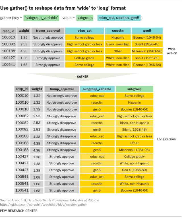
## 6 100039 6.68 Strongly disappro… High school gra… Black, non… Boomer (1…The next step is to rearrange the data in a way that makes it easy to calculate the weighted summary statistics by each demographic group. We’ll do this with the gather() function, which reshapes data from “wide” format to “long” — an extremely useful function when working with data. (Recently, the team behind the tidyr package introduced functions called pivot_longer() and pivot_wider(). These functions will not replace gather() and spread(), but are designed to be more useful and intuitive.)
In wide format, there is one row per person and one column per variable. In long format, there are multiple rows per person: one for each of the demographic variables we want to analyze. The separate demographic columns are replaced by a pair of columns; a “key” column and a “value” column. Here, the “key” column is called subgroup_variable, and it identifies which demographic variable is associated with that row (one of educ_cat, racethn, or gen5). The “value” column is called subgroup and identifies the specific demographic category to which the person belongs.
Apr17_long <- Apr17 %>%
gather(key = subgroup_variable, value = subgroup,
educ_cat, racethn, gen5)
In this code, we’re telling gather() to name the key variable "subgroup_variable" and to name the value column "subgroup." The remaining arguments specify the names of the columns that we want to gather into rows. After the gather() step, we’ve gone from a wide dataset with 1,501 rows to a long dataset 4,503 rows (1,501 respondents x 3 demographic variables).
If you want to read more about gather(), I recommend starting with this tweetby Alison Hill from the WeAreRLadies twitter account. You can also go to the tidy data chapter in the previously mentioned R for Data Science book.
Now that we have our data arranged in this format, getting weighted summaries for all three subgroup variables is just a matter adding another grouping variable. Whereas before we grouped by educ_cat, we can now use our newly created subgroup_variable and subgroup columns instead.
trump_estimates <- Apr17_long %>%
#group by subgroup_variable, subgroup, and trump approval
group_by(subgroup_variable, subgroup, trump_approval) %>%
#calculate the total number of people in each answer and education #category using survey weights (weight)
summarise(weighted_n = sum(weight)) %>%
#group by subgroup only to calculate subgroup category size
group_by(subgroup) %>%
#add columns for total group size and the proportion
mutate(weighted_group_size = sum(weighted_n),
weighted_estimate = weighted_n/weighted_group_size)
Since we are only really interested in the proportions, we’ll remove the weighted_total and weighted_group_size columns using the select() function. Including the — before a column name tells select() to drop that column.
trump_estimates <- trump_estimates %>%
select(-weighted_n, -weighted_group_size)
Here’s what we end up with.
trump_estimates
## # A tibble: 70 x 4
## # Groups: subgroup [14]
## subgroup_variable subgroup trump_approval weighted_estima…
##     <chr>               <chr>                <fct>              <dbl>
## 1 educ_cat           College grad+      Strongly approve        0.267
## 2 educ_cat           College grad+      Not strongly appr…     0.0715
## 3 educ_cat           College grad+      Not strongly disa…     0.0870
## 4 educ_cat           College grad+      Strongly disappro…      0.537
## 5 educ_cat           College grad+          Refused            0.0373
## 6 educ_cat         Don't know/Refuse…   Strongly approve       0.0203
## 7 educ_cat         Don't know/Refuse…   Strongly disappro…     0.0704
## 8 educ_cat         High school grad …   Strongly approve        0.322
## 9 educ_cat         High school grad …   Not strongly appr…      0.121
## 10 educ_cat        High school grad …   Not strongly disa…      0.129
## # … with 60 more rows
Arranging the data this way makes it easy to create plots or tables of the variables of interest. Below is an example of a simple plot of the estimates we created in this post. We use the filter() function to remove the “Refused” category in the trump_approval variable and in any of our subgroup variables. Then, we pipe that data into the plotting code from ggplot2.
trump_estimates %>%
filter(trump_approval != "Refused") %>%
filter(!(subgroup %in%
c("Don't know/Refused (VOL.)", "DK/Ref"))) %>%
ggplot(
aes(
x = weighted_estimate,
y = subgroup
)
) +
geom_point() +
scale_x_continuous(limits = c(0, .8),
breaks = seq(0, .6, by = .2),
labels = scales::percent(
seq(0, .6, by = .2), accuracy = 1)
) +
facet_grid(cols = vars(trump_approval),
rows = vars(subgroup_variable),
scales = "free_y",
space = "free"
) +
theme_bw() +
theme(axis.title.y = element_blank())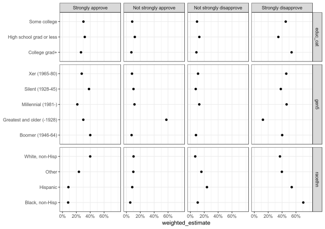
Here is all the necessary code used in the post:
#code from start to finish

##install or update packages if neccessary
#install.packages("tidyverse")
#install.packages("haven")

##load packages in
library(tidyverse) #loads all "core" tidyverse packages like dplyr, tidyr, forcats, and ggplot2
library(haven)

##read dataset in with value labels (as_factor)
Apr17 <- read_sav("Apr17 public.sav", user_na = TRUE) %>% as_factor()

##create trump_approval variable and relevel it
Apr17 <- Apr17 %>%
  mutate(trump_approval = case_when(
    q1 == "Approve" & q1a == "Very strongly" ~ "Strongly approve",
    q1 == "Approve" & q1a != "Very strongly" ~ "Not strongly approve",
    q1 == "Disapprove" & q1a == "Very strongly" ~ "Strongly disapprove",
    q1 == "Disapprove" & q1a != "Very strongly" ~ "Not strongly disapprove",
    q1 == "Don't know/Refused (VOL.)" | q1a == "Don't know/Refused (VOL.)" ~ "Refused"
  ) #this parentheses closes our call to case_when
  %>% #and then sends it to fct_relevel with %>%
    fct_relevel("Strongly approve",
                "Not strongly approve",
                "Not strongly disapprove",
                "Strongly disapprove",
                "Refused"
    ) #this parentheses closes our call to fct_relevel
  ) #this parentheses closes our call to mutate

## collapse education variable into 3 categories
Apr17 <- Apr17 %>%
  mutate(educ_cat = fct_collapse(educ2,
                                 "High school grad or less" = c(
                                   "Less than high school (Grades 1-8 or no formal schooling)",
                                   "High school incomplete (Grades 9-11 or Grade 12 with NO diploma)",
                                   "High school graduate (Grade 12 with diploma or GED certificate)"
                                 ),
                                 "Some college" = c(
                                   "Some college, no degree (includes some community college)",
                                   "Two year associate degree from a college or university"
                                 ),
                                 "College grad+" = c(
                                   "Four year college or university degree/Bachelor's degree (e.g., BS, BA, AB)",
                                   "Some postgraduate or professional schooling, no postgraduate degree",
                                   "Postgraduate or professional degree, including master's, doctorate, medical or law degree"
                                 )
  ) #this parentheses closes our call to fct_collapse
  ) #this parentheses closes our call to mutate

##get trump_approval weighted totals
trump_approval <- Apr17 %>%
  group_by(trump_approval) %>%
  summarise(weighted_n = sum(weight))

##get trump_approval weighted proportions
trump_approval <- Apr17 %>%
  ##group by trump_approval to calculated weighted totals by taking the sum of the weights
  group_by(trump_approval) %>%
  summarise(weighted_n = sum(weight)) %>%
  ##add the weighted_group_size to get the total weighted n and
  ##divide weighted_n by weighted_group_size to get the proportions
  mutate(weighted_group_size = sum(weighted_n),
         weighted_estimate = weighted_n / weighted_group_size
  )


##get trump_approval by education
trump_estimates_educ <- Apr17 %>%
  #group by educ and trump approval to get weighted n's per group
  group_by(educ_cat, trump_approval) %>%
  #calculate the total number of people in each answer and education category using survey weights (weight)
  summarise(weighted_n = sum(weight)) %>%
  #group by education to calculate education category size
  group_by(educ_cat) %>%
  #add columns for total group size and the proportion
  mutate(weighted_group_size = sum(weighted_n),
         weighted_estimate = weighted_n/weighted_group_size)

##select only columns interested in for this analysis
###rename psraid to resp_id
Apr17 <- Apr17 %>%
  select(resp_id = psraid, weight, trump_approval, educ_cat, racethn, gen5)

##create Apr_17 long with gather
Apr17_long <- Apr17 %>%
  #gather educ_cat, racethn, gen5 into two columns:
  ##a key  called "subgroup variable" (educ_cat, racethn, gen5)
  ##and a value called "subgroup"
  gather(key = subgroup_variable, value = subgroup, educ_cat, racethn, gen5)

##get weighted estimates for every subgroup
trump_estimates <- Apr17_long %>%
  #group by subgroup_variable, subgroup, and trump approval to get weighted n of approval/disapproval for all subgroup cats
  group_by(subgroup_variable, subgroup, trump_approval) %>%
  #calculate the total number of people in each answer and education category using survey weights (weight)
  summarise(weighted_n = sum(weight)) %>%
  #group by subgroup only to calculate subgroup category size
  group_by(subgroup) %>%
  #add columns for total group size and the proportion
  mutate(weighted_group_size = sum(weighted_n),
         weighted_estimate = weighted_n/weighted_group_size)

#only want proportions so select out total categories
trump_estimates <- trump_estimates %>%
  select(-weighted_n, -weighted_group_size)

##create plot
trump_estimates %>%
  ##remove "Refused" category for Trump Approval
  filter(trump_approval != "Refused") %>%
  ##remove Refused categories in our subgroup values
  filter(!(subgroup %in% c("Don't know/Refused (VOL.)", "DK/Ref"))) %>%
  ggplot(
    aes(
      x = weighted_estimate,
      y = subgroup
    )
  ) +
  geom_point() +
  scale_x_continuous(limits = c(0, .8),
                     breaks = seq(0, .6, by = .2),
                     labels = scales::percent(seq(0, .6, by = .2), accuracy = 1)
  ) +
  facet_grid(cols = vars(trump_approval),
             rows = vars(subgroup_variable),
             scales = "free_y",
             space = "free"
  ) +
  theme_bw() +
  theme(axis.title.y = element_blank())


