In 2017, Pew Research Center published an analysis of Google search trendsrelated to the water crisis in Flint, Michigan. The analysis used the Google Health Application Programming Interface (API) to examine search patterns within the Flint media market, the state of Michigan and across the United States. The study marked the first time the Center used data like these, and because of the interest the project drew from other researchers, we published guidelines for how to use search data in general and the Google Health API data in particular (in addition to a statement describing our methodology).
As the Center explores new datasets and methods, we want to allow other researchers to replicate and build on our work. Today, in a step toward that goal, we are releasing our code publicly for the first time — beginning with the code we used to conduct our Flint research.
There are two main components to the code we are releasing today: a custom-written Python module called search_sampler that retrieves data from the Health API (given an approved key) and a set of R scripts that we used to clean and analyze that data for the published report.
Today’s code release will be followed by others in the coming months. We are excited to use GitHub to share resources with new audiences, staying true to our mission of informing the public while also showing how we do the work we do. You can find our GitHub page here, and you can use the comments section below or email info@pewresearch.org with any questions about our repositories or code.
Repositories used in Flint study
About search_sampler
Search_sampler is a Python module that queries the Google Health API for search data and saves the results in a .csv file in the location specified.
About the Google Health API
The Google Health API is one of three public tools Google offers to examine search data; the others are the Google Trends website and the Google Trends API (you can learn more about the differences here). Access to the Google Health API requires approval; the application to the Google Health API can be found here.
The Health API requires a set of search terms (keywords used in people’s searches; for information on selecting terms, see here) and can be limited to a specific time range and geography. At the time of analysis, the geographic area of interest can be constrained to the country, state, or Designated Market Area (DMA) level for queries related to searches in the United States. The API then returns a series of values for these specified search terms within that time range and geography. The result is a series of data points, each of which is based on the search volume at a specified interval, which can be daily, weekly or monthly. (In our Flint report, we used weekly data.)
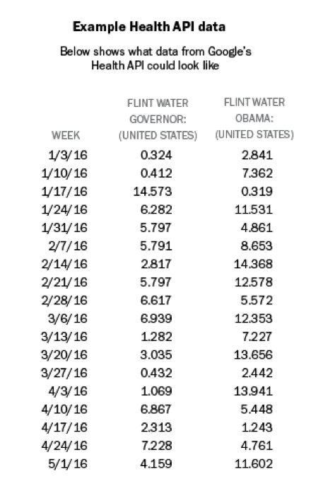
One key aspect of all search volume results is that they are presented as scaled proportions, not as absolute numbers of searches. The scaled proportion is the number of searches with the specified keywords during that interval and in the geographic area specified, divided by the total number of searches during that interval in that geographic area. This proportion is then multiplied by a constant number. Although Google does not publish what that number is, it is consistent across queries to the Health API, which allows for comparison across queries. For example, if you send a request to the Health API for all searches that contain the keywords “flint water governor” in the U.S. during 2016 at weekly intervals, the result will be a series of values for each week in 2016. Below is a sample of what this result would look like, using artificial, not actual, data:

Because the number of searches conducted by the public is very large, the Health API does not actually conduct a census of all searches. Instead, when retrieving search results, it first samples the full set of search results, and the results the API actually analyzes and returns are from this sample, not the full results. A new sample is drawn approximately every 24 hours. This means that the same query will return different results if repeated on different days.
To reduce this sampling error, search_sampler gives users the option to repeat the same query numerous times on different samples. The package submits a series of queries using the chosen search terms for different, overlapping time ranges. Because each query covers a different time period, each one relies on a different sample from the full database. This eliminates the need to wait 24 hours before repeating any given query and maximizes the number of values that can be sampled at a time. For instance, if a researcher is looking at a 20-week period, this program can break that five-month block into four-week chunks. It would then call the API several times: The first would be weeks 1–4, the second would be weeks 2–5, then weeks 3–6, and so on. When it concludes, each week will have four samples instead of just one. (The sliding window actually starts before your start date and finishes after your end date, so each time period — weeks, in this case — is sampled the same number of times.) All data are compiled into the same file, which can then be analyzed using the R scripts below.
Particularly rare search terms introduce an additional complication. If a given sample does not contain enough searches that match the specified keywords, it will return 0 instead of the actual number. This does not mean that the true number of searches at that time was zero, but that the number of searches was too small to report without jeopardizing the privacy of Google’s users. For search terms that are right on the border of this threshold, repeated queries will return a mixture of positive values and zeroes that need to be handled in the analysis (see an example below). To address this in our Flint study, we used 50 distinct samples.
Using search_sampler
This package can be installed using pip:
pip install search_samplerUsing search_sampler is straightforward. First assign your API key and specify a path to the folder where you want to save the results, which will be output as .csv files. Then specify the parameters you want to use: the search term(s), the region, the start and end dates, and whether you want data at the daily, weekly or monthly levels. These will be passed into the search_sampler class as a dictionary, along with your API key, output path and a unique name that will be associated with your search parameters and the name of the output file.
apikey = ‘’
output_path = ‘’ # Folder name in your current directory to save results. This will be created.
search_name = ‘My Search Name’# search params
params = {
# Can be any number of search terms, using Boolean logic. See report methodology for more info.
  ‘search_term’:[‘cough’],

  # Can be country, state, or DMA. States are US-CA. DMA are a 3 digit code; see Nielsen for info.
  ‘region’:’US-DC’,  # Must be in format YYYY-MM-DD
  ‘period_start’:’2014–01–01',
  ‘period_end’:’2014–02–15',  # Options are day, week, month. WARNING: This has been extensively tested with week only.
  ‘period_length’:’week’
}
sampler = search_sampler(apikey, search_name, params,
  output_path=output_path)
Once you have set up the search_samplerinstance, you can either run a single sample:
df_results = sample.pull_data_from_api()Or a rolling set of samples:
df_results = sample.pull_rolling_window(num_samples=num_samples)Once concluded, save your sample using the save_files command:
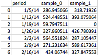
sample.save_file(df_results)An example of a resulting data file is below (again based on a simulation, not actual data). Each rolling window sample is shown in a column, and each row is an interval of data. Note the variability of the data across the same time periods and the presence of zero values — data points in which the privacy threshold was not met.

Flint water R repository — Searching_for_news
For our study of the Flint water crisis, we used search_sampler to get weekly trends for five different categories of search terms for the period of Jan. 5, 2014, to July 2, 2016, for the entire United States, the state of Michigan and the Flint DMA. For each combination of geography and search terms, we used 50 unique samples. Once downloaded, we performed our analysis in R. The code we used is in the Flint water repository, available here.
The code consists of two scripts, each of which handles different steps of the analysis. For the scripts to work, there should be a separate directory for each geography containing .csv files for each set of search terms.
The first script is impute_samples.r, which takes the raw data from search_sampler and gets it into shape for the main analysis of search trends. Most of the work is done by the combine_category() function. This takes the results for each of the 50 samples for a given set of search terms in a geography and averages them. Any duplicate samples are removed. Then, any zero values that were returned by the API are imputed. Finally, the values for each week are averaged across all of the samples. The result is a single time series where sampling error and zero values have been largely removed, which can be analyzed using standard tools.
The second script, create_changepoints.r, helps identify inflection points when the rate of search volume changes. It is not always clear when these changes are meaningful. To identify meaningful shifts in searches, we first eliminated noise using a smoothing technique called a generalized additive model. We then identified broad periods (several weeks or months) in which the number of searches was different from the periods around it using a changepoint model, and we compared the peaks between these periods.
For more details on why we chose this approach, please see our longer post here.
Using R methods
Combining samples
After we drew samples using the process above, we combined them into single values for each data point. To do so, however, we first imputed the values of data points with a zero value. We performed this imputation through a mixed effects model that incorporated the average value of the samples that did not have a zero for that data point as well as the other values of that sample.
To create just a single sample, use the impute_samples.r script. There are three important functions in this script: dedupe(), which removes any duplicate columns (something that can happen if you do not wait long enough between re-running search_sampler), combine_category(), and combine_region().
To use this script, first set the main directory in which your data are stored. This should not be the final directory in which the data are stored, but its parent directory. This design was adopted so users could run multiple regions, all in different subfolders, without resetting the parent directory. (The default behavior in the sampling package above is to save data for each region sampled in a folder named after the region under the main folder.)
Call process_region() with this parent directory and the name of the region:
starting_dir = <main data folder>
combine_region(starting_dir, ‘513’)
This will scan the folder for any .csv files and run them through combine_category(), which performs the imputation. It then takes the mean for each data point and saves the result in a single .csv file for each category in a combined subfolder.
Creating changepoints
At this point users will have a results file with the imputed mean value for each period, as well as many of the data used to generate those means (original mean, logged version, qq value, etc.). The next step is to create the changepoints, which is done in the create_changepoints.r file.
The majority of this work is done in the run_plots() function, which reads the mean values for each data point, smooths the dataset using a generalized additive model, and runs a changepoint analysis using the changepoint package(along with a graph showing the initial changepoints). The resulting data files and changepoints are saved in a changepoint folder under the main data folder.
To call run_plots(), pass the name of the folder containing the combined data produced above and the name of the region as you would want it to appear in charts:
run_plots(“<folder>”, “Flint”)Much of this work is actually done in the cp_binseg() function, which is called by run_plots().
First, smoothing is performed using a generalized additive model, which predicts the value for a given data point using the mean of the imputed value across samples.
# calculate means
df_means = df %>%
  group_by(period_date) %>%
  summarize(imputed_mean = mean(imputed_value))# run gam
m = gam(imputed_value~s(num_period, k=k_val),  data=df)# get predicted values
df_pred = df %>%
  select(period_date, num_period) %>%
  distinct() %>%
  as_tibble()df_pred$smoothed = predict(m, newdata = df_pred)
Second, changepoints are identified using the binary segmentation method in the changepoint package. After setting up the data, running the changepoint requires just a few lines:
# Run model and put results in a list
binseg_est = cpt.mean(df_means$imputed_mean, method=”BinSeg”, Q=Q_val, minseglen = 3)
Finally, the mean and max of each period, as well as the difference between periods, is calculated for graphing and analysis, and the final data and charts are saved in the changepoint folder.
We hope this explainer has been useful. If you end up using these scripts for your own research, or have any questions, we’d love to hear from you. You can reach us by commenting on this post, emailing us at info@pewresearch.org, or talking to us on Twitter via @PewMethods.


