The survey literature has long shown that more respondents say they intend to vote than actually cast a ballot (e.g., Bernstein et al. 2001; Silver et al. 1986). In addition, some people say they do not expect to vote but actually do, perhaps because they are contacted by a campaign or a friend close to Election Day and are persuaded to turn out. These situations potentially introduce error into election forecasts because these stealth voters and nonvoters often differ in their partisan preferences. In general, Republicans are more likely than Democrats to turn out, though they may be about equally likely to say they intend to vote. As a consequence, pollsters do not rely solely upon a respondent’s stated intention when classifying a person as likely to vote or not. Instead, most ask several questions that collectively can be used to estimate an individual’s likelihood of voting. The questions measure intention to vote, past voting behavior, knowledge about the voting process and interest in the campaign.

This study examines different ways of using seven standard questions, and sometimes other information, to produce a model of the likely electorate. The questions were originally developed in the 1950s and ’60s by election polling pioneer Paul Perry of Gallup and have been used – in various combinations and with some alterations – by Pew Research Center, Gallup and other organizations in their pre-election polling (Perry 1960, 1979). The questions tested here include the following (the categories that give a respondent a point in the Perry-Gallup index, discussed in the following section, are in bold):

• How much thought have you given to the coming November election? Quite a lot, some, only a little, none
• Have you ever voted in your precinct or election district? Yes, no
• Would you say you follow what’s going on in government and public affairs most of the time, some of the time, only now and then, hardly at all?
• How often would you say you vote? Always, nearly always, part of the time, seldom
• How likely are you to vote in the general election this November? Definitely will vote, probably will vote, probably will not vote, definitely will not vote
• In the 2012 presidential election between Barack Obama and Mitt Romney, did things come up that kept you from voting, or did you happen to vote? Yes, voted; no
• Please rate your chance of voting in November on a scale of 10 to 1. 0-8, 9, 10

Some pollsters have employed other kinds of variables in their likely voter models, including demographic characteristics, partisanship and ideology. Below we evaluate models that use these types of measures as well.

Two additional kinds of measures tested here are taken from a national voter file. These include indicators for past votes (in 2012 and 2010) and a predicted turnout score that synthesizes past voting behavior and other factors to produce an estimated likelihood of voting. These measures are strongly associated with voter turnout. A detailed analysis of all of these individual measures and how closely each one is correlated with voter turnout and vote choice can be found in Appendix A to this report.

Two broad approaches are used to produce a prediction of voting with pre-election information such as the Perry-Gallup questions or self-reported past voting history (Burden 1997). Deterministic methods use the information to categorize each survey respondent as a likely voter or nonvoter, typically dividing voters and nonvoters using a threshold or “cutoff” that matches the predicted rate of voter turnout in the election. Probabilistic methods use the same information to compute the probability that each respondent will vote. Probabilities can be used to weight respondents by their likelihood of voting, or they can be used as a basis for ranking respondents for a cutoff approach. This analysis examines the effectiveness of both approaches.

The Perry-Gallup likely voter index

Following the original method developed by Paul Perry, Pew Research Center combines the individual survey items to create a scale that is then used to classify respondents as likely voters or nonvoters. For each of the seven questions, a respondent is given 1 point for selecting certain response categories. For example, a response of “yes” to the question “Have you ever voted in your precinct or election district?” gets 1 point on the scale. Younger respondents are given additional points to account for their inability to vote in the past (respondents who are ages 20-21 get 1 additional point and respondents who are ages 18-19 get 2 additional points).⁶ Additionally, those who say they “definitely will not” be voting, or who are not registered to vote, are automatically coded as a zero on the scale. As tested here, the procedure results in an index with values ranging from 0 to 7, with the highest values representing those with the greatest likelihood of voting.

The next step is to make an estimate of the percentage of the eligible adults likely to vote in the election. This is typically based on a review of past turnout levels in similar elections, adjusted for judgments about the apparent level of voter interest in the current campaign, the competitiveness of the races and degree of voter mobilization underway. The estimate is used to produce a “cutoff” on the likely voter scale, selecting the highest-scoring respondents based on the expected turnout in the coming election. For example, if we expected that 40% of the voting eligible population would vote (a typical turnout for a midterm election), then we would base our survey estimates on the 40% of the eligible public receiving the highest index scores.⁷ In reality, 36% of the eligible adult population turned out in 2014. The choice of a turnout threshold is a very important decision because the views of voters and nonvoters are often very different, as was the case in 2014. (See Appendix C for data on how the choice of a turnout target matters.)⁸

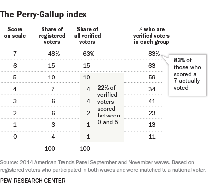
Deterministic (or cutoff) methods like this one leave out many actual voters. While those coded 6 and 7 on the scale are very likely to vote (63% and 83% of each group, respectively were validated to have voted), there also are many actual voters among those who scored below 6: About a fifth (22%) of all verified voters scored between 0 and 5. Of course, the goal of the model is not to classify every respondent but to produce an accurate aggregation of the vote. But if the distribution of those correctly classified does not match that of the actual electorate, the election forecast will be wrong.

Consistent with general patterns observed in previous elections of this type, respondents who scored a 7 on the scale favor Republican over Democratic candidates (by a margin of 50% to 44%). Majorities of those in categories 5 and 6 prefer Democratic candidates. As in most elections, the partisan distribution of the predicted vote depends heavily on where the line is drawn on the likely voter scale. Including more voters usually makes the overall sample more Democratic, especially in off-year elections. That is why judgments about where to apply the cutoff are critical to the accuracy of the method.

Probabilistic models

The same individual survey questions can also be used to create a statistical model that assigns a predicted probability of voting to each respondent, along with coefficients that measure how well each item correlates with turnout. These coefficients can then be used in other elections with surveys that ask the same questions to create a predicted probability of voting for each respondent, based on the assumption that expressions of interest, past behavior and intent all have the same impact regardless of the election. All response options for each item can be used in the model, or they can be coded as they are in the Perry-Gallup method. Regardless of the form of the inputs, the result is a distribution, with each respondent assigned a score on a scale corresponding to how likely he or she is to turn out to vote. If someone is classified as a 0.30, then that respondent is thought to have a 30% chance of voting.

One potential benefit to this method is that it can use more of the information contained in the survey (all of the response categories in each question, rather than just a selected one or two). This also gives respondents who may have a lower likelihood of voting – whether because of their age, lack of ongoing interest in the election or simply having missed a past election – a possibility of affecting the outcome, since we know that many who score lower on the scale actually do vote. These respondents will be counted as long as they have a chance of voting that is greater than zero; they are simply given a lower weight in the analysis than others with a higher likelihood of voting.

One potential drawback of this method is that it applies a model developed in a previous election to a current election, based on the assumption that the relationships between turnout and the key predictors are the same across elections. In this study, our models are built using voter participation data from the 2014 elections, and the resulting weights are applied retroactively to produce survey estimates of the likely 2014 vote. As a result, we cannot test how well these models would perform in future elections. The likely voter model used by CBS News, which has employed a variation of this method for decades, suggests that such assumptions are reasonable. Rather, our goal is to explore the differences between probabilistic and deterministic approaches to modeling voter turnout, and learn how much these models are improved when we include information on prior voting behavior drawn from the voter file.

In our evaluations of probabilistic models, we also tested a “kitchen sink” model that includes the seven Perry-Gallup measures along with a range of demographic and political variables including age, education, income, race/ethnicity, party affiliation, ideological consistency, home ownership and length of tenure at current residence – all factors known to be correlated with voter turnout.

In testing probabilistic approaches, we explored two methods for creating predicted probabilities: logistic regression, a common modeling tool, and a machine-learning technique known as “random forest.”

In addition to using the predicted probabilities as a weight, they can also be used with a cutoff. As with the Perry-Gallup scale, the cutoff method would count the top-scoring respondents as likely voters and ignore the others. For example, assuming that 60% of registered voters are going to turn out, the models would include only the top 60% of respondents as ranked by their predicted probabilities of voting.

Logistic regression

To build a model comparable to the Perry-Gallup seven-item scale, the same seven questions on voter engagement, past voting behavior, voter intent and knowledge about where to vote were used. (The “kitchen sink” model used these items along with demographic and political variables.) The questions were entered into the model as predictors without combining or collapsing categories. Variables were rescaled to vary between 0 and 1, with “don’t know” responses coded as zero.

A logistic regression was performed using verified vote from the voter file as the dependent variable. The regression produces a predicted probability of voting for each respondent and coefficients for each measure. The probabilities are then used in various ways as described below to produce a model of the electorate for forecasting. In subsequent elections, the coefficients derived from these models can be used with the answers from respondents in contemporary surveys to produce a probability of voting for each person. As with the Perry-Gallup approach, this method assumes that the measures used in the study are equally relevant for distinguishing voters from nonvoters in a variety of elections.

Decision trees and random forests

Another probabilistic approach involves the use of “decision trees” to identify the best configuration of variables to predict a particular outcome – in this case, voting and nonvoting. The typical decision tree analysis identifies various ways of splitting a dataset into separate paths or branches, based on options for each variable. The decision tree approach can be improved using a machine-learning technique known as “random forests.” Random forests employ large numbers of trees fit to random subsamples of the data in order to provide more precise predictions than would be obtained by fitting a single tree to all of the data. Unlike classical methods for estimating probabilities such as logistic regression, random forests perform well with large numbers of predictor variables and in the presence of complex interactions. We applied the random forest method to the computation of vote probabilities, starting with the same variables employed in the other methods described earlier.

When a single decision tree is fit to a dataset, the algorithm starts by searching for the value among the predictor variables that can be used to split the dataset into two groups that are most homogenous with respect to the outcome variable, in this case whether or not someone voted in the 2014 elections. These subgroups are called nodes, and the decision tree algorithm proceeds to split each node into progressively more and more homogenous groups until a stopping criterion is reached. One thing that makes the random forest technique unique is that prior to splitting each node, the algorithm selects a random subset of the predictor variables to use as candidates for splitting the data. This has the effect of reducing the correlation between individual trees, which further reduces the variance of the predictions.

When employing statistical models for prediction, it is important to address the possibility that the models are overfitting the data – finding patterns in data that reflect random noise rather than meaningful signal – which reduces their accuracy when applied to other datasets. This is less of a concern for logistic regression, which is unlikely to overfit when the sample size is large relative to the number of independent variables (as is the case here). But it is a concern for powerful machine-learning methods such as random forests that actively seek out patterns in data. One advantage of random forests in this regard is the fact that each tree is built using a different random subsample of the data. In our analysis, the predicted probabilities for a case are based only on those trees that were built using subsamples where that case was excluded. The result is that any overfitting that occurs in the tree-building process does not carry over into the scores that are applied to each case.

One final regression-based method tested here is to employ a voter turnout probability created by the voter file vendor as a predictor or a weight. The TargetSmart voter file includes a 2014 turnout likelihood score developed by Clarity Campaign Labs. This score ranges from 0 to 1 and can be interpreted as a probability of voting in the 2014 general election.

The statistical analysis reported in the next section uses the verified vote as the measure of turnout. Among registered voters in the sample, 63% have a voter file record indicating that they voted in 2014. Self-reported voting was more common; 75% of registered voters said they turned out. Appendix B discusses the pros and cons of using verified vote vs. self-reported vote.